Function Reference: leasqr

Function File: leasqr (x, y, pin, F)

Function File: leasqr (x, y, pin, F, stol)

Function File: leasqr (x, y, pin, F, stol, niter)

Function File: leasqr (x, y, pin, F, stol, niter, wt)

Function File: leasqr (x, y, pin, F, stol, niter, wt, dp)

Function File: leasqr (x, y, pin, F, stol, niter, wt, dp, dFdp)

Function File: leasqr (x, y, pin, F, stol, niter, wt, dp, dFdp, options)

Function File: [f, p, cvg, iter, corp, covp, covr, stdresid, Z, r2] = leasqr (…)

Levenberg-Marquardt nonlinear regression.

Input arguments:

x

Vector or matrix of independent variables.

y

Vector or matrix of observed values.

pin

Vector of initial parameters to be adjusted by leasqr.

F

Name of function or function handle. The function must be of the form y = f(x, p), with y, x, p of the form y, x, pin.

stol

Scalar tolerance on fractional improvement in scalar sum of squares, i.e., sum ((wt .* (y-f))^2). Set to 0.0001 if empty or not given;

niter

Maximum number of iterations. Set to 20 if empty or not given.

wt

Statistical weights (same dimensions as y). These should be set to be proportional to sqrt (y) ^-1, i.e., the covariance matrix of the data is assumed to be proportional to diagonal with diagonal equal to (wt.^2)^-1. The constant of proportionality will be estimated. Set to ones (size (y)) if empty or not given.

dp

Fractional increment of p for numerical partial derivatives. Set to 0.001 * ones (size (pin)) if empty or not given.

dp(j) > 0 means central differences on j-th parameter p(j).
dp(j) < 0 means one-sided differences on j-th parameter p(j).
dp(j) = 0 holds p(j) fixed, i.e., leasqr won’t change initial guess: pin(j)

dFdp

Name of partial derivative function in quotes or function handle. If not given or empty, set to dfdp, a slow but general partial derivatives function. The function must be of the form prt = dfdp (x, f, p, dp, F [,bounds]). For backwards compatibility, the function will only be called with an extra ’bounds’ argument if the ’bounds’ option is explicitly specified to leasqr (see dfdp.m).

options

Structure with multiple options. The following fields are recognized:

fract_prec: Column vector (same length as pin) of desired fractional precisions in parameter estimates. Iterations are terminated if change in parameter vector (chg) relative to current parameter estimate is less than their corresponding elements in ’fract_prec’, i.e., all (abs (chg) < abs (options.fract_prec .* current_parm_est)) on two consecutive iterations. Defaults to zeros (size (pin)).
max_fract_change: Column vector (same length as pin) of maximum fractional step changes in parameter vector. Fractional change in elements of parameter vector is constrained to be at most ’max_fract_change’ between sucessive iterations, i.e., abs (chg(i)) = abs (min([chg(i), options.max_fract_change(i) * current param estimate])). Defaults to Inf * ones (size (pin)).
inequc: Cell-array containing up to four entries, two entries for linear inequality constraints and/or one or two entries for general inequality constraints. Initial parameters must satisfy these constraints. Either linear or general constraints may be the first entries, but the two entries for linear constraints must be adjacent and, if two entries are given for general constraints, they also must be adjacent. The two entries for linear constraints are a matrix (say m) and a vector (say v), specifying linear inequality constraints of the form ‘m.’ * parameters + v >= 0’. If the constraints are just bounds, it is suggested to specify them in ’options.bounds’ instead, since then some sanity tests are performed, and since the function ’dfdp.m’ is guarantied not to violate constraints during determination of the numeric gradient only for those constraints specified as ’bounds’ (possibly with violations due to a certain inaccuracy, however, except if no constraints except bounds are specified). The first entry for general constraints must be a differentiable vector valued function (say h), specifying general inequality constraints of the form ‘h (p[, idx]) >= 0’; p is the column vector of optimized paraters and the optional argument idx is a logical index. h has to return the values of all constraints if idx is not given, and has to return only the indexed constraints if idx is given (so computation of the other constraints can be spared). If a second entry for general constraints is given, it must be a function (say dh) which returnes a matrix whos rows contain the gradients of the constraint function h with respect to the optimized parameters. It has the form jac_h = dh (vh, p, dp, h, idx[, bounds]); p is the column vector of optimized parameters, and idx is a logical index — only the rows indexed by idx must be returned (so computation of the others can be spared). The other arguments of dh are for the case that dh computes numerical gradients: vh is the column vector of the current values of the constraint function h, with idx already applied. h is a function h (p) to compute the values of the constraints for parameters p, it will return only the values indexed by idx. dp is a suggestion for relative step width, having the same value as the argument ’dp’ of leasqr above. If bounds were specified to leasqr, they are provided in the argument bounds of dh, to enable their consideration in determination of numerical gradients. If dh is not specified to leasqr, numerical gradients are computed in the same way as with ’dfdp.m’ (see above). If some constraints are linear, they should be specified as linear constraints (or bounds, if applicable) for reasons of performance, even if general constraints are also specified.
bounds: Two-column-matrix, one row for each parameter in pin. Each row contains a minimal and maximal value for each parameter. Default: [-Inf, Inf] in each row. If this field is used with an existing user-side function for ’dFdp’ (see above) the functions interface might have to be changed.
equc: Equality constraints, specified the same way as inequality constraints (see field ’options.inequc’). Initial parameters must satisfy these constraints. Note that there is possibly a certain inaccuracy in honoring constraints, except if only bounds are specified. Warning: If constraints (or bounds) are set, returned guesses of corp, covp, and Z are generally invalid, even if no constraints are active for the final parameters. If equality constraints are specified, corp, covp, and Z are not guessed at all.
cpiv: Function for complementary pivot algorithm for inequality constraints. Defaults to cpiv_bard. No different function is supplied.

For backwards compatibility, options can also be a matrix whose first and second column contains the values of fract_prec and max_fract_change, respectively.

Output:

f: Column vector of values computed: f = F(x,p).
p: Column vector trial or final parameters, i.e, the solution.
cvg: Scalar: = 1 if convergence, = 0 otherwise.
iter: Scalar number of iterations used.
corp: Correlation matrix for parameters.
covp: Covariance matrix of the parameters.
covr: Diag(covariance matrix of the residuals).
stdresid: Standardized residuals.
Z: Matrix that defines confidence region (see comments in the source).
r2: Coefficient of multiple determination, intercept form.

Not suitable for non-real residuals.

References: Bard, Nonlinear Parameter Estimation, Academic Press, 1974. Draper and Smith, Applied Regression Analysis, John Wiley and Sons, 1981.

Demonstration 1

The following code

 % Define functions
 leasqrfunc = @(x, p) p(1) * exp (-p(2) * x);
 leasqrdfdp = @(x, f, p, dp, func) [exp(-p(2)*x), -p(1)*x.*exp(-p(2)*x)];

 % generate test data
 t = [1:10:100]';
 p = [1; 0.1];
 data = leasqrfunc (t, p);
 
 rnd = [0.352509; -0.040607; -1.867061; -1.561283; 1.473191; ...
        0.580767;  0.841805;  1.632203; -0.179254; 0.345208];

 % add noise
 % wt1 = 1 /sqrt of variances of data
 % 1 / wt1 = sqrt of var = standard deviation
 wt1 = (1 + 0 * t) ./ sqrt (data); 
 data = data + 0.05 * rnd ./ wt1; 

 % Note by Thomas Walter :
 %
 % Using a step size of 1 to calculate the derivative is WRONG !!!!
 % See numerical mathbooks why.
 % A derivative calculated from central differences need: s 
 %     step = 0.001...1.0e-8
 % And onesided derivative needs:
 %     step = 1.0e-5...1.0e-8 and may be still wrong

 F = leasqrfunc;
 dFdp = leasqrdfdp; % exact derivative
 % dFdp = dfdp;     % estimated derivative
 dp = [0.001; 0.001];
 pin = [.8; .05]; 
 stol=0.001; niter=50;
 minstep = [0.01; 0.01];
 maxstep = [0.8; 0.8];
 options = [minstep, maxstep];

 global verbose;
 verbose = 1;
 [f1, p1, kvg1, iter1, corp1, covp1, covr1, stdresid1, Z1, r21] = ...
    leasqr (t, data, pin, F, stol, niter, wt1, dp, dFdp, options);

Produces the following output

Least Squares Estimates of Parameters
   1.0050   0.1026
 Correlation matrix of parameters estimated
   1.0000   0.5745
   0.5745   1.0000
 Covariance matrix of Residuals
   2.6477e-03
   9.7403e-04
   3.5832e-04
   1.3182e-04
   4.8494e-05
   1.7840e-05
   6.5629e-06
   2.4144e-06
   8.8820e-07
   3.2675e-07
 Correlation Coefficient R^2
0.9983
 95% conf region: F(0.05)(2,8)>= delta_pvec.'*Z*delta_pvec
Z =

   1.8909e+02  -1.2096e+03
  -1.2096e+03   2.3441e+04

and the following figure

Figure 1

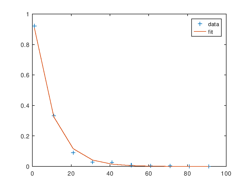Demonstration 2

The following code

  %% Example for linear inequality constraints.
  %% model function:
  F = @ (x, p) p(1) * exp (p(2) * x);
  %% independents and dependents:
  x = 1:5;
  y = [1, 2, 4, 7, 14];
  %% initial values:
  init = [.25; .25];
  %% other configuration (default values):
  tolerance = .0001;
  max_iterations = 20;
  weights = ones (1, 5);
  dp = [.001; .001]; % bidirectional numeric gradient stepsize
  dFdp = "dfdp"; % function for gradient (numerical)

  %% linear constraints, A.' * parametervector + B >= 0
  A = [1; -1]; B = 0; % p(1) >= p(2);
  options.inequc = {A, B};

  %% start leasqr, be sure that 'verbose' is not set
  global verbose; verbose = false;
  [f, p, cvg, iter] = ...
      leasqr (x, y, init, F, tolerance, max_iterations, ...
	      weights, dp, dFdp, options)

Produces the following output

f =

    1.1536    2.1451    3.9891    7.4179   13.7941

p =

   0.6203
   0.6203

cvg = 1
iter = 7

and the following figure

Figure 1

Package: optim