- Function File:
[p, s] =wpolyfit(x, y, dy, n)¶ Return the coefficients of a polynomial p(x) of degree n that minimizes
sumsq (p(x(i)) - y(i)), to best fit the data in the least squares sense. The standard error on the observations y if present are given in dy.The returned value p contains the polynomial coefficients suitable for use in the function polyval. The structure s returns information necessary to compute uncertainty in the model.
To compute the predicted values of y with uncertainty use
[y,dy] = polyconf(p,x,s,'ci');
You can see the effects of different confidence intervals and prediction intervals by calling the wpolyfit internal plot function with your fit:
feval('wpolyfit:plt',x,y,dy,p,s,0.05,'pi')Use dy=[] if uncertainty is unknown.
You can use a chi^2 test to reject the polynomial fit:
p = 1-chi2cdf(s.normr^2,s.df);
p is the probability of seeing a chi^2 value higher than that which was observed assuming the data are normally distributed around the fit. If p < 0.01, you can reject the fit at the 1% level.
You can use an F test to determine if a higher order polynomial improves the fit:
[poly1,S1] = wpolyfit(x,y,dy,n);
[poly2,S2] = wpolyfit(x,y,dy,n+1);
F = (S1.normr^2 - S2.normr^2)/(S1.df-S2.df)/(S2.normr^2/S2.df);
p = 1-f_cdf(F,S1.df-S2.df,S2.df);
p is the probability of observing the improvement in chi^2 obtained by adding the extra parameter to the fit. If p < 0.01, you can reject the lower order polynomial at the 1% level.
You can estimate the uncertainty in the polynomial coefficients themselves using
dp = sqrt(sumsq(inv(s.R'))'/s.df)*s.normr;
but the high degree of covariance amongst them makes this a questionable operation.
- Function File:
[p, s, mu] =wpolyfit(...)¶ -
If an additional output
mu = [mean(x),std(x)]is requested then the x values are centered and normalized prior to computing the fit. This will give more stable numerical results. To compute a predicted y from the returned model usey = polyval(p, (x-mu(1))/mu(2)
- Function File: wpolyfit
(...)¶ -
If no output arguments are requested, then wpolyfit plots the data, the fitted line and polynomials defining the standard error range.
Example
x = linspace(0,4,20);
dy = (1+rand(size(x)))/2;
y = polyval([2,3,1],x) + dy.*randn(size(x));
wpolyfit(x,y,dy,2);
- Function File: wpolyfit
(..., 'origin')¶ -
If ’origin’ is specified, then the fitted polynomial will go through the origin. This is generally ill-advised. Use with caution.
Hocking, RR (2003). Methods and Applications of Linear Models. New Jersey: John Wiley and Sons, Inc.
See also: core Octave
polyfit.See also: polyconf.
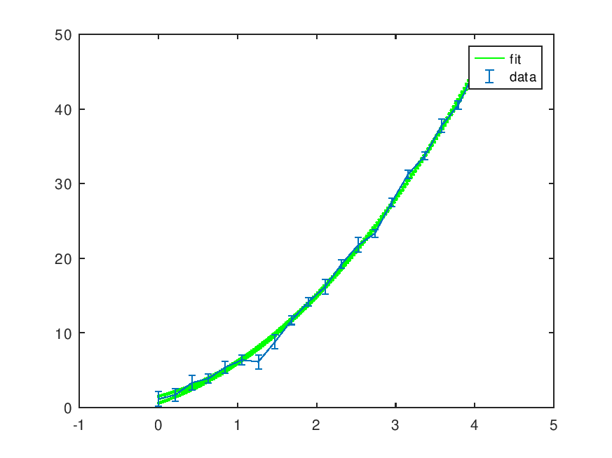
Demonstration 1
The following code
 % #1
 x = linspace(0,4,20);
 dy = (1+rand(size(x)))/2;
 y = polyval([2,3,1],x) + dy.*randn(size(x));
 wpolyfit(x,y,dy,2);
Produces the following output
Polynomial: 1.8202*x^2 + 3.5661*x^1 + 0.90708  [ p(chi^2>observed)=43.31% ]
See residuals? [y,n] y
and the following figure
| Figure 1 |
|---|
 |
Demonstration 2
The following code
 % #2
 x = linspace(-i,+2i,20);
 noise = ( randn(size(x)) + i*randn(size(x)) )/10;
 P = [2-i,3,1+i];
 y = polyval(P,x) + noise;
 wpolyfit(x,y,2)
Produces the following output
Polynomial: (2.0014-0.95997i)*x^2 + (3.0441-0.027627i)*x^1 + (0.97157+1.0531i) [ p(chi^2>observed)=100.00% ]
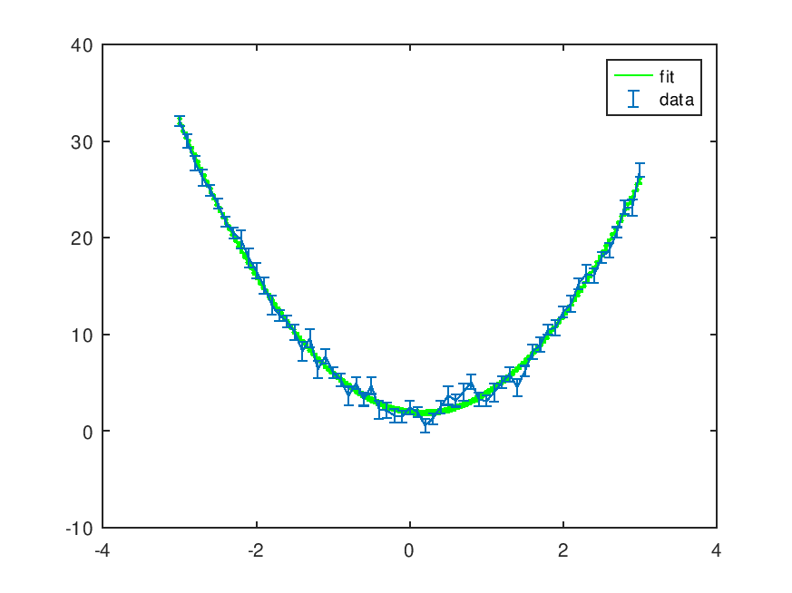
Demonstration 3
The following code
 pin = [3; -1; 2];
 x = -3:0.1:3;
 y = polyval (pin, x);

 ## Poisson weights
 # dy = sqrt (abs (y));
 ## Uniform weights in [0.5,1]
 dy = 0.5 + 0.5 * rand (size (y));

 y = y + randn (size (y)) .* dy;
 printf ("Original polynomial: %s\n", polyout (pin, 'x'));
 wpolyfit (x, y, dy, length (pin)-1);
Produces the following output
Original polynomial: 3*x^2 - 1*x^1 + 2
Polynomial: 3.0417*x^2 - 0.97091*x^1 + 1.8196  [ p(chi^2>observed)=27.82% ]
See residuals? [y,n] y
and the following figure
| Figure 1 |
|---|
 |
Package: optim