- Function File: M = ctmctaexps (Q, t, p0)
- Function File: M = ctmctaexps (Q, p0)
-
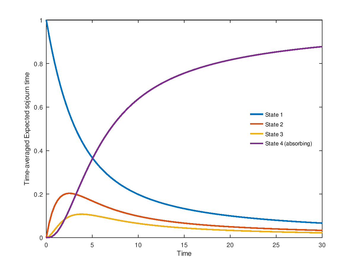
Compute the time-averaged sojourn time
M(i), defined as the fraction of the time interval [0,t] (or until absorption) spent in state i, assuming that the state occupancy probabilities at time 0 are p.INPUTS
Q(i,j)Infinitesimal generator matrix.
Q(i,j)is the transition rate from state i to state j, 1 ≤ i,j ≤ N, i \neq j. The matrix Q must also satisfy the condition \sum_{j=1}^N Q_{i,j} = 0tTime. If omitted, the results are computed until absorption.
p0(i)initial state occupancy probabilities.
p0(i)is the probability that the system is in state i at time 0, i = 1, …, N
OUTPUTS
M(i)When called with three arguments,
M(i)is the expected fraction of the interval [0,t] spent in state i assuming that the state occupancy probability at time zero is p. When called with two arguments,M(i)is the expected fraction of time until absorption spent in state i; in this case the mean time to absorption issum(M).
See also: ctmcexps.
Demonstration 1
The following code
 lambda = 0.5;
 N = 4;
 birth = lambda*linspace(1,N-1,N-1);
 death = zeros(1,N-1);
 Q = diag(birth,1)+diag(death,-1);
 Q -= diag(sum(Q,2));
 t = linspace(1e-5,30,100);
 p = zeros(1,N); p(1)=1;
 M = zeros(length(t),N);
 for i=1:length(t)
   M(i,:) = ctmctaexps(Q,t(i),p);
 endfor
 clf;
 plot(t, M(:,1), ";State 1;", "linewidth", 2, ...
      t, M(:,2), ";State 2;", "linewidth", 2, ...
      t, M(:,3), ";State 3;", "linewidth", 2, ...
      t, M(:,4), ";State 4 (absorbing);", "linewidth", 2 );
 legend("location","east"); legend("boxoff");
 xlabel("Time");
 ylabel("Time-averaged Expected sojourn time");
Produces the following figure
| Figure 1 |
|---|
 |
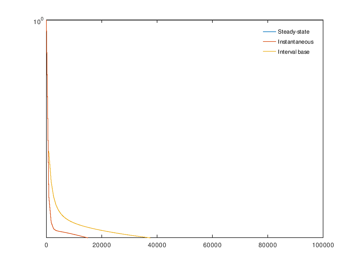
Demonstration 2
The following code
 sec = 1;
 min = sec*60;
 hour = 60*min;
 day = 24*hour;

 # state space enumeration {2, RC, RB, 1, 0}
 a = 1/(10*min);    # 1/a = duration of reboot (10 min)
 b = 1/(30*sec);    # 1/b = reconfiguration time (30 sec)
 g = 1/(5000*hour); # 1/g = processor MTTF (5000 hours)
 d = 1/(4*hour);    # 1/d = processor MTTR (4 hours)
 c = 0.9;           # coverage
 Q = [ -2*g 2*c*g 2*(1-c)*g      0  0; ...
          0    -b         0      b  0; ...
          0     0        -a      a  0; ...
          d     0         0 -(g+d)  g; ...
          0     0         0      d -d];
 p = ctmc(Q);
 printf("System availability: %f\n",p(1)+p(4));
 TT = linspace(0,1*day,101);
 PP = ctmctaexps(Q,TT,[1 0 0 0 0]);
 A = At = Abart = zeros(size(TT));
 A(:) = p(1) + p(4); # steady-state availability
 for n=1:length(TT)
   t = TT(n);
   p = ctmc(Q,t,[1 0 0 0 0]);
   At(n) = p(1) + p(4); # instantaneous availability
   Abart(n) = PP(n,1) + PP(n,4); # interval base availability
 endfor
 clf;
 semilogy(TT,A,";Steady-state;", ...
      TT,At,";Instantaneous;", ...
      TT,Abart,";Interval base;");
 ax = axis();
 ax(3) = 1-1e-5;
 axis(ax);
 legend("boxoff");
Produces the following output
System availability: 0.999989
and the following figure
| Figure 1 |
|---|
 |
Package: queueing