Function Reference: qncsmvaap

Function File: [U, R, Q, X] = qncsmvaap (N, S, V)

Function File: [U, R, Q, X] = qncsmvaap (N, S, V, m)

Function File: [U, R, Q, X] = qncsmvaap (N, S, V, m, Z)

Function File: [U, R, Q, X] = qncsmvaap (N, S, V, m, Z, tol)

Function File: [U, R, Q, X] = qncsmvaap (N, S, V, m, Z, tol, iter_max)

Analyze closed, single class queueing networks using the Approximate Mean Value Analysis (MVA) algorithm. This function is based on approximating the number of customers seen at center k when a new request arrives as Q_k(N) \times (N-1)/N. This function only handles single-server and delay centers; if your network contains general load-dependent service centers, use the function qncsmvald instead.

INPUTS

N: Population size (number of requests in the system, N > 0).
S(k): mean service time on server k (S(k)>0).
V(k): average number of visits to service center k (V(k) ≥ 0).
m(k): number of servers at center k (if m is a scalar, all centers have that number of servers). If m(k) < 1, center k is a delay center (IS); if m(k) == 1, center k is a regular queueing center (FCFS, LCFS-PR or PS) with one server (default). This function does not support multiple server nodes (m(k) > 1).
Z: External delay for customers (Z ≥ 0). Default is 0.
tol: Stopping tolerance. The algorithm stops when the maximum relative difference between the new and old value of the queue lengths Q becomes less than the tolerance. Default is 10^{-5}.
iter_max: Maximum number of iterations (iter_max>0. The function aborts if convergenge is not reached within the maximum number of iterations. Default is 100.

OUTPUTS

U(k): If k is a FCFS, LCFS-PR or PS node (m(k) == 1), then U(k) is the utilization of center k. If k is an IS node (m(k) < 1), then U(k) is the traffic intensity defined as X(k)*S(k).
R(k): response time at center k. The system response time Rsys can be computed as Rsys = N/Xsys - Z
Q(k): average number of requests at center k. The number of requests in the system can be computed either as sum(Q), or using the formula N-Xsys*Z.
X(k): center k throughput. The system throughput Xsys can be computed as Xsys = X(1) / V(1)

REFERENCES

This implementation is based on Edward D. Lazowska, John Zahorjan, G. Scott Graham, and Kenneth C. Sevcik, Quantitative System Performance: Computer System Analysis Using Queueing Network Models, Prentice Hall, 1984. http://www.cs.washington.edu/homes/lazowska/qsp/. In particular, see section 6.4.2.2 ("Approximate Solution Techniques").

See also: qncsmva,qncsmvald.

Demonstration 1

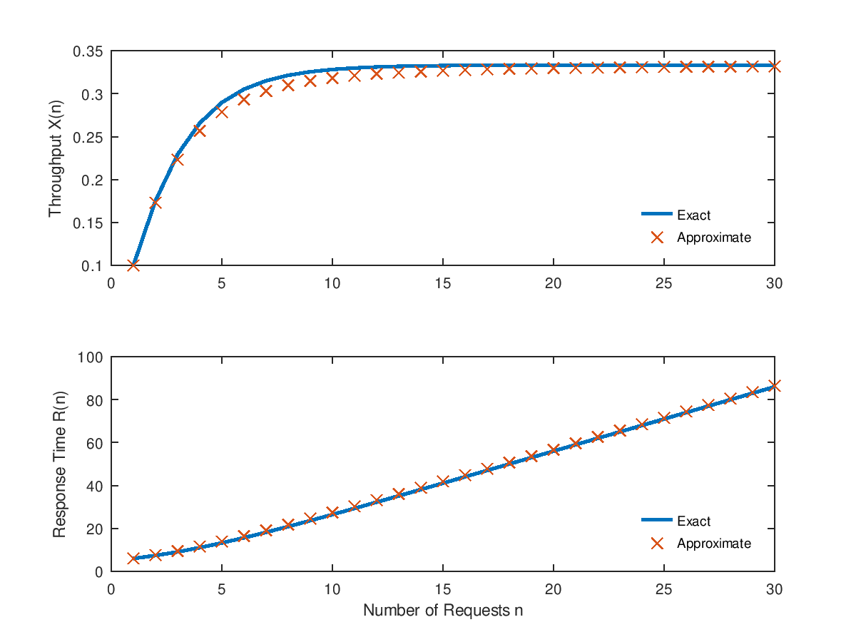
The following code

 S = [ 0.125 0.3 0.2 ];
 V = [ 16 10 5 ];
 N = 30;
 m = ones(1,3);
 Z = 4;
 Xmva = Xapp = Rmva = Rapp = zeros(1,N);
 for n=1:N
   [U R Q X] = qncsmva(n,S,V,m,Z);
   Xmva(n) = X(1)/V(1);
   Rmva(n) = dot(R,V);
   [U R Q X] = qncsmvaap(n,S,V,m,Z);
   Xapp(n) = X(1)/V(1);
   Rapp(n) = dot(R,V);
 endfor
 subplot(2,1,1);
 plot(1:N, Xmva, ";Exact;", "linewidth", 2, 1:N, Xapp, "x;Approximate;", "markersize", 7);
 legend("location","southeast"); legend("boxoff");
 ylabel("Throughput X(n)");
 subplot(2,1,2);
 plot(1:N, Rmva, ";Exact;", "linewidth", 2, 1:N, Rapp, "x;Approximate;", "markersize", 7);
 legend("location","southeast"); legend("boxoff");
 ylabel("Response Time R(n)");
 xlabel("Number of Requests n");

Produces the following figure

Figure 1

Package: queueing