Chapter 1. OCT Files
Octahedron, octopus, oculist, oct-file? – What?
An oct-file is a dynamical extension of the Octave interpreter, in other words a shared library or shared object. The source files, that make up an oct-file, are written in C++, and therefore, conventionally, carry the extension cc.
Why would you ever want to write in C++ again, having the wonderful Octave environment at your service? Well, sometimes the performance of native Octave-code is not enough to attack a problem. Octave-code is interpreted, thus it is inherently slow when executed (especially if the problem cannot be vectorised). In such a case moving from m-code to compiled C++-code speeds up the execution by a factor of ten or more. The second group of problems, where reverting to low-level code is necessary, is when interfacing with foreign libraries (think of LAPACK) or routines written in languages other than C++, most notably Fortran-77.
Having convinced ourselves that we have to bite the bullet, we start with an easy tutorial (Section 1.1). This will teach any reader who is sufficiently used to C++ how to write her first dynamically linked extension for Octave. Having guided the reader with her first steps, Section 1.2 covers more advanced topics of writing extensions. For later reference, we provide a quick reference of the most helpful methods of the Octave interface classes in Section 1.3.
1.1. Tutorial
The tutorial unfurls slowly; we do not want to scare anybody by the complexity of the task ahead. At any time, if you feel like it, look into the directories OCT/src or OCT/src/DLD-FUNCTIONS, where OCT is the root directory of your Octave source-tree and consult the header-files and already existent dynamic extensions.
1.1.1. Problem Definition
Instead of giving an abstract treatise, we want to explain the whole business of dynamical extensions with the help of a simple, yet non-trivial problem. This example shall be analyzed in detail from beginning to end, and we shall elucidate some modern software construction principles on the way.
We shall implement a matrix power function.[1] Given a square
matrix A of integers, reals, or complex
values, and a non-negative integral
exponent n, the
function matpow(A,
n) is to calculate
An.
We have to watch out for boundary cases: an empty matrix A or a zero exponent n.
1.1.2. High-Level Implementation
We postpone writing the C++-implementation until we are completely satisfied with our implementation in Octave. Having Octave, a rapid prototyping environment at hand, it would be stupid to throw away its possibilities.
Hobby Astronomer's Mirror Making Rule
It is faster to grind a 3 inch mirror and then a 5 inch mirror, that to grind a 5 inch mirror.
Now that the problem is exactly defined, we can start thinking about an implementation. Here is our naive first shot:
Example 1-1. Naive implementation of matpow
function b = matpow0(a, n)
    ## Return b = a^n for square matrix a, and non-negative, integral n.
    ## Note: matpow0() is an extremely naive implementation.

    b = diag(ones(size(a, 1), 1));
    for i = 1:n
        b = b * a;
    endfor
endfunction
Easy does the job! matpow0 looks like it does what we
want, but how can we be sure? We write a test-suite[2]! A test-suite is
needed when we switch to C++. We have a piece of running code, so
let us write some tests. The unit testing functions are defined in Appendix A, Section A.1.
### name:        test_matpow.m  --  test matrix power functions
### original:    Ch. L. Spiel

###
### The following tests should succeed.
###

unit_init(0, {"a"}); ## Quiet testing, use global variable a

a = [ 2.0, -3.0;
     -1.0,  1.0];

unit_test_equals("a^0",  matpow0(a, 0), diag([1, 1]));
unit_test_equals("a^1",  matpow0(a, 1), a);
unit_test_equals("a^2",  matpow0(a, 2), a^2);
unit_test_equals("a^3",  matpow0(a, 3), a^3);
unit_test_equals("a^4",  matpow0(a, 4), a^4);
unit_test_equals("a^22", matpow0(a, 22), a^22);
unit_test_equals("a^23", matpow0(a, 23), a^23);

###
### print results
###

unit_results();
Running the tests on matpow0 gives us confidence
octave:2> test_matpow
................
# of testcases attempted   7
# of expected passes       7
# of expected failures     0
# of unexpected passes     0
# of unexpected failures   0
# of unresolved testcases  0
but we also get more ambitious!
Our algorithm is really naive, and matrix multiplications are computationally expensive. Let us cut down on the number of multiplications. What is the minimum number of multiplications needed to compute An? Starting with A, we can only square it, getting A2. Again squaring is the fastest way to get to the fourth power. In general squaring our highest power lets us avance with least multiplications. This is the heart of our new algorithm.
Improved matrix power algorithm. If the exponent n is a w-bit number, we can apply the binary expansion n = sum(bi * 2i, i = 0..w-1), where the bi are either 0 or 1. In other words, we square A for every bit in the binary expansion of n, multiplying this value with the final result if bi = 1. Special care has to be taken for the cases where n = 0 or 1. See also [Golub:1996], section 11.2.5, page 569.
Example 1-2. Implementation of improved matrix power algorithm
function b = matpow1(a, n)
    ## Return b = a^n for square matrix a, and non-negative, integral n.

    -- handle special cases: n = 0, and n = 1
    -- first, to allow for an early return
    if (n == 0)
        b = diag(ones(size(a, 1), 1));
        return;
    endif

    if (n == 1)
        b = a;
        return;
    endif

    -- general case: n >= 2
    p = a;                              -- p holds the current square
    b = a;
    np = n - 1;
    while (np >= 1)
        if (is_even(np))                -- is_even is defined below
            -- zero in the binary expansion
            np = np / 2;
        else
            -- one in the binary expansion
            np = (np - 1) / 2;
            b *= p;
        endif
        p *= p;
    endwhile
endfunction


function e = is_even(n)
    ## Return true (1), if n is even, false (0) otherwise.

    e = (rem(n, 2) == 0)
endfunction
The new algorithm reduces the number of matrix multiplications from O(n), to O(log2(n)), which is a remarkable improvement for large matrices as matrix multiplication itself is an O(m3) process (m is the number of rows and columns of the matrix).
Running the test-suite again ensures that we did not code any nonsense.
1.1.3. Our First Dynamic Extension
Ready for the jump to light speed? Wait – we have to feed the navigation computer first!
1.1.3.1. Feature Compatibility
In principle, the functions defined in oct-files must have the same capabilities as functions in m-files. In particular, the input and output arguments lists must be able to carry different numbers of arguments, which are moreover of different type, just as m-file functions can. This means that there must be a way of mapping a function from Octave like
function [array, real-scalar, integer] =
    func(complex-scalar, array, list, integer)
    ## func frobs the snafu, returning all gromniz coefficients.

    -- actual function code goes here

endfunction
to C++. To this end, Octave's core interface supplies the macro (in OCT/src/defun-int.h)
octave_value_list
DEFUN_DLD(function_name,
          const octave_value_list& input_argument_list,
          [ int number_of_output_arguments ],            -- optional argument
          const char* documentation_string)
We have decorated the macro arguments with their types. Note that the first argument is the name of the function to be defined.
Of course the macro has to be defined somewhere. The easiest way to pull in all necessary definitions is to include OCT/src/oct.h. Now, our skeletal source file of the dynamic extension has the following shape:
#include <oct.h>

DEFUN_DLD(func, args, nargout,
          "func frobs the snafu, returning the gromniz coefficients.")
{
    -- actual function code goes here

    return possibly_empty_list_of_values;
}
Often functions do not depend on the actual number of output parameters.
Then, the third argument to DEFUN_DLD
can be omitted.
 | Naming convention |
|---|---|
|
1.1.3.2. Essential types and methods
Before we start to write a low-level implementation of
matpow, we look at the most essential types
and methods used to handle data that flows through the
Octave-interpreter interface.
As has been said above, the arguments passed to dynamically loaded
functions are bundled in an octave_value_list. Results
returned from a function are also passed in an
octave_value_list. The default constructor,
octave_value_list, creates an empty list which,
when used as return value, yields an Octave function returning
"void". To access the elements of a list the following methods
form class octave_value_list (defined in
OCT/src/oct-obj.h) are useful:
{
public octave_value_list();public octave_value& operator()(int index);  public const octave_value operator()(int index);  public const int length();}
length returns the number of elements in
the list. The overloaded parenthesis operator selects a single
element from the list. The index base for
index is 0 and not
1 as Fortran adepts might infer. The value returned by
operator() is an
octave_value, i.e., any type known to Octave,
e.g. integers, real matrices, complex matrices, and so on.
Knowing how to access the arguments of unspecified type, the next thing we would like to do is get their values. Octave follows a uniform naming scheme: all functions that return an object of a certain type ends in _type. Some of the more important of these methods (defined in OCT/src/ov-base.h) are:
{
public const int int_value();  public const double double_value();  public const Complex complex_value();  public const Matrix matrix_value();  public const ComplexMatrix complex_matrix_value();}
1.1.3.3. Low-level implementation
Now, we are ready to implement matpow as a dynamically
loaded extension to Octave.
Example 1-3. C++ implementation of matpow
#include <octave/oct.h>
static bool is_even(int n);
DEFUN_DLD(matpow, args, ,
"Return b = a^n for square matrix a, and non-negative, integral n.")
{
const int n = args(1).int_value();  if (n == 0)
return octave_value(
DiagMatrix(args(0).rows()
if (n == 0)
return octave_value(
DiagMatrix(args(0).rows() , args(0).columns()
 , 1.0)
  );
if (n == 1)
return args(0);
Matrix p(args(0).matrix_value());
);
if (n == 1)
return args(0);
Matrix p(args(0).matrix_value());  Matrix b(p);
int np = n - 1;
while (np >= 1)
{
if (is_even(np))
{
np = np / 2;
}
else
{
np = (np - 1) / 2;
b = b * p;
Matrix b(p);
int np = n - 1;
while (np >= 1)
{
if (is_even(np))
{
np = np / 2;
}
else
{
np = (np - 1) / 2;
b = b * p;  }
p = p * p;
}
return octave_value(b);
}
p = p * p;
}
return octave_value(b);  }
bool
is_even(int n)
{
return n % 2 == 0;
}
}
bool
is_even(int n)
{
return n % 2 == 0;
}
- Get the exponent
n, which is the second argument tomatpowthroughargs(1) and retrieve its integral value withint_value. - The matrix that we want to raise to the n-th power is the
first argument, therefore it is accessed
through
args(0). The methodrowsreturns the number of rows in the matrix. - The method
columnsreturns the number of columns in the matrix. (The actual value is assumed to be equal to the number of rows. At this stage, we are tacitly assuming that all parameters passed tomatpoware valid, which means especially that the matrix is square.) - We call a constructor for diagonal matrices,
DiagMatrix(defined in OCT/liboctave/dDiagMatrix.h), that accepts the size of the matrix and the value to put on the diagonal, which is 1 in our case. - Initialise the matrix
pthat will store the powers of the base. TheMatrixconstructor cannot take an octave_value and we have to supply the matrix itself by invokingmatrix_value. - Multiplication has been conveniently overloaded to work on matrices. Wanna give John a treat for this one?
- We can return the result matrix
bdirectly, as an appropriate constructor is invoked to convert it to an octave_value_list.
| The Octave library overloads all elementary operations of scalars, (row-/column-) vectors and matrices. If in doubt as to whether a particular operation has been overloaded, simply try it. It takes less time than browsing (read: grep through) all the sources – the desired elementary operation is implemented in most cases. |
We learn from the example that the C++ closely resembles the Octave function. This is due to the clever class structure of the Octave library.
1.1.3.4. Compiling
Now that we are done with the coding, we are ready to compile and link. The Octave distribution contains the script mkoctfile, which does exactly this for us. In the simplest case it is called with the C++-source as its only argument.
$ ls
Makefile  matpow0.m  matpow1.m  matpow.cc  test_matpow.m
$ mkoctfile matpow.cc
Good, but not good enough! Presumably, we shall compile several times, so we would like to run our test suite and finally remove all files that can be re-generated from source. Enter: Makefile.
1.1.3.5. Running
If the oct-file is in the LOADPATH, it
will be loaded automatically – either when requesting
help on the function or when invoking it directly.
$ ls
Makefile  matpow0.m  matpow1.m  matpow.cc  matpow.o  matpow.oct  test_matpow.m
$ octave -q
octave:1> help matpow
matpow is the dynamically-linked function from the file
/home/cspiel/hsc/octave/src/matpow/matpow.oct

Return b = a^n for square matrix a, and non-negative, integral n.

octave:2> matpow([2, 0; 0, -1], 4)
ans =

  16   0
   0   1

octave:3> Ctrl-D
1.1.4. Spicing up matpow
The keen reader will have noticed that matpow is
highly vulnerable to unexpected input. We take care of this deficiency in
Section 1.1.4.1.
Also, the documentation is not ready for prime time, something we
attend to in Section 1.1.4.2.
1.1.4.1. Input parameter checking
Why do we need parameter checking at all? A rule of thumb is to perform a complete parameter checking on
every function that is exposed to the user (e.g. at Octave's interpreter level), i.e. for every function created with
DEFUN_DLD, orany function that might be used in a different context than the writer intended Functions that are used only internally do not require full parameter checking.
One problem which arises frequently with parameter checking of (interfacing) functions is that the checks easily take up more space than the routine itself, thereby distracting the reader from the function's original purpose. Often, including all the checks into the main function bloats it beyond the desired maintainability. Therefore, we have to take precautions against these problems by consistently factoring out all parameter checks.
The rule of thumb here is to group logically related tests together in separate functions. The testing functions get the original functions' arguments by constant reference and return a boolean value. Constant referencing avoids any constructor calls and – in addition to that – protects the arguments against modification. In our example a single test function is enough:
static bool any_bad_argument(const octave_value_list& args);
any_bad_argument prints a detailed message, raises an
Octave error, and returns true if the arguments fail
any test; otherwise it returns false and we can
continue processing. The only thing we have to change in
matpow is to add a call to
any_bad_argument and on failure to return an Octave-void
value, i.e. an empty octave_value_list. The first few lines
of matpow then take the following form:
DEFUN_DLD(matpow, args, ,
          "Return b = a^n for square matrix a, and non-negative, integral n.")
{
    if (any_bad_argument(args))
        return octave_value_list();

    const int n = args(1).int_value();

    -- rest of matpow is unchanged
}
As we are convinced that we have to check the input arguments, the question is how to do the checks.
| Ordering of Tests |
|---|---|
The correct ordering of tests is essential!
Item 1 always goes first. Items 2-4 usually repeat for each of the arguments. The final tests check the relations between the arguments, i.e., belong to Item 5. |
Octave supplies the user with all necessary type- and size-testing functions. The type-tests (defined in OCT/src/ov-base.h) share the common prefix is_. Here are the most commonly used:
{
public const bool is_real_scalar();  public const bool is_complex_scalar();  public const bool is_real_matrix();  public const bool is_complex_matrix();}
To examine the sizes of different Octave objects, the following methods prove useful:
{
public const int length();}
{
public const int rows(); public const int columns(); public const int length();}Remember that the methods available depend on the underlying type. For example, a ColumnVector only has a length (OCT/src/ov-list.h), whereas a Matrix has a number of rows and columns (OCT/src/ov-base-mat.h).
We have all the knowledge we need to write the argument testing function to
augment matpow.
static bool
any_bad_argument(const octave_value_list& args)
{
    if (!args(0).is_real_matrix())
    {
        error("matpow: expecting base A (arg 1) to be a real matrix");
        return true;
    }

    if (args(0).rows() != args(0).columns())
    {
        error("matpow: expecting base A (arg 1) to be a square matrix");
        return true;
    }

    if (!args(1).is_real_scalar())
    {
        error("matpow: exponent N (arg 2) must be a real scalar.");
        return true;
    }

    if (args(1).scalar_value() < 0.0)
    {
        error("matpow: exponent N (arg 2) must be non-negative.");
        return true;
    }

    if (floor(args(1).scalar_value()) != args(1).scalar_value())
    {
        error("matpow: exponent N (arg 2) must be an integer.");
        return true;
    }

    return false;
}
Out final duty is to update the test-frame and run it. For brevity, we only list the new tests in testmp.m
###
### The following tests should trigger the error exits.
###

## number of arguments

unit_test_err("error exit, too few arguments",
              "matpow:", "matpow([1,1; 1,1])");

unit_test_err("error exit, too few arguments",
              "matpow:", "matpow()");

unit_test_err("error exit, too many arguments",
              "matpow:", "matpow([1,1; 1 1], 2, 1)");

## argument type and size

unit_test_err("error exit, A not a matrix",
              "matpow:", "matpow(1, 1)");

unit_test_err("error exit, A not a square matrix",
              "matpow:", "matpow([1 2 3; 4 5 6], 1)");

unit_test_err("error exit, N not a real scalar(here: complex)",
              "matpow:", "matpow(a, 1+i)");

unit_test_err("error exit, N not a real scalar(here: non-scalar)",
              "matpow:", "matpow(a, ones(2,2))");

unit_test_err("error exit, N negative",
              "matpow:", "matpow(a, -1)");

unit_test_err("error exit, N non-integral",
              "matpow:", "matpow(2.5)");
$ octave -q test_matpow.m
................
# of testcases attempted   16
# of expected passes       16
# of expected failures     0
# of unexpected passes     0
# of unexpected failures   0
# of unresolved testcases  0

Unit testing completed successfully!
1.1.4.2. Texinfo documentation strings
Our much improved matpow still carries around the poor
documentation string:
"Return b = a^n for square matrix a, and non-negative, integral n."
Let us improve on this one! Octave supports documentation strings – docstrings for short – in Texinfo format. The effect on the online documentation will be small, but the appearance of printed documentation will be greatly improved.
The fundamental building block of Texinfo documentation strings is the Texinfo-macro @deftypefn, which takes two arguments: The class the function is in, and the function's signature. For functions defined with DEFUN_DLD, the class is Loadable Function. A skeletal Texinfo docstring therefore looks like this:
Example 1-5. Skeletal Texinfo Docstring
-*- texinfo -*-
- Tell the parser that the doc-string is in Texinfo format.
- @deftypefn{class} ... @end deftypefn encloses the whole doc-string, like a LaTeX environment or a DocBook element does.
- @cindex index entry generates an index entry. It can be used multiple times.
Texinfo has several macros which control the markup. In the group of format changing commands, we note @var{variable_name}, and @code{code_piece}. The Texinfo format has been designed to generate output for online viewing with text-terminals as well as generating high-quality printed output. To these ends, Texinfo has commands which control the diversion of parts of the document into a particular output processor. Two formats are of importance: info and TeX. The first is selected with
@ifinfo
text for info only
@end ifinfo
the latter with
@iftex
@tex
text for TeX only
@end tex
@end iftex
If no specific output processor is chosen, by default, the test goes into both (or, more precisely: every) output processors. Usually, neither @ifinfo, nor @iftex appear alone, but always in pairs, as the same information must be conveyed in every output format.
Example 1-6. Documentation string in Texinfo format
-*- texinfo -*-
@deftypefn{Loadable Function} {@var{b} =} matpow(@var{a}, @var{n})

@cindex matrix power

Return matrix @var{a} raised to the @var{n}-th power.  Matrix @var{a} is
a square matrix and @var{n} a non-negative integer.
@iftex
@tex
$n = 0$
@end tex
@end iftex
@ifinfo
n = 0
@end ifinfo
is explicitly allowed, returning a unit-matrix of the same size as
@var{a}.

Note: @code{matpow}  duplicates part of the functionality of the built-in
exponentiation operator
@iftex
@tex
``$\wedge$''.
@end tex
@end iftex
@ifinfo
`@code{^}'.
@end ifinfo


Example:
@example
matpow([1, 2; 3, 4], 4)
@end example
@noindent
returns
@example
ans =

  199  290
  435  634
@end example

The algorithm takes
@iftex
@tex
$\lfloor \log_{2}(n) \rfloor$
@end tex
@end iftex
@ifinfo
floor(log2(n))
@end ifinfo
matrix multiplications to compute the result.
@end deftypefn
- @iftex ... @end iftex selects text for conditional inclusion. Only if the text is processed with an Tex the included section will be processed.
- @tex ... @end tex wraps parts of the text that will be fed through TeX.
- @ifdoc ... @end ifdoc selects text for conditional inclusion. Only if the text is processed with an info-tool the included section will be processed.
- @code{code sequence} marks up a a code sequence.
- @example ... @end example wraps examples.
For further information about Texinfo consult the Texinfo documentation. For TeX-beginners we recommend "The Not So Short Introduction to LaTeX" by Tobias Oetiker et. al.
One thing we held back is the true appearance of a Texinfo docstring – mainly because it looks so ugly. The C++-language imposes the constraint that the docstring must be a string-constant. Moreover, because DEFUN_DLD is a macro, every line-end has to be escaped with a backslash. The backslash does not insert any whitespace and TeX separates paragraphs with empty lines, so that we have to put in new-lines as line-separators. Thus, the Texinfo docstring in source form has each line end decorated with "\n\".
DEFUN_DLD(matpow, args, ,
          "-*- texinfo -*-\n\
@deftypefn{Loadable Function} {@var{b}} = matpow(@var{a}, @var{n})\n\
\n\
@cindex matrix power\n\
\n\
Return matrix @var{a} raised to the @var{n}-th power.  Matrix @var{a} is\n\
a square matrix, and @var{n} a non-negative integer.\n\
...")
At least the formatted versions look much better. The info-version, which will be used in Octave's online help has approximately the following appearance:
b = matpow(a, n)                                        Loadable Function
Return matrix a raised to the n-th power. Matrix a is a square matrix, and
n a non-negative integer. n = 0 is explicitely allowed, returning a
unit-matrix of the same size as a.

Note: matpow duplicates part of the functionality of the built-in
exponentiation operator `^'.

Example:
matpow([1, 2; 3, 4], 4)

returns
ans =

  199  290
  435  634

The algorithm takes floor(log2(n)) matrix multiplications to compute the
result.
whereas the TeX-version will look like this:
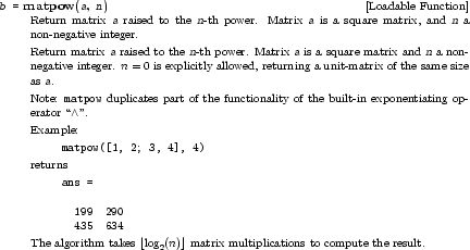
Docstring of matpow after rendering with TeX.
Note the differences between the info-version and the TeX-version,
that have been introduced with @ifinfo and
@iftex.