- Function File: impulse (sys)
- Function File: impulse (sys1, sys2, …, sysN)
- Function File: impulse (sys1, 'style1', …, sysN, 'styleN')
- Function File: impulse (sys1, …, t)
- Function File: impulse (sys1, …, tfinal)
- Function File: impulse (sys1, …, tfinal, dt)
- Function File: [y, t, x] = impulse (sys)
- Function File: [y, t, x] = impulse (sys, t)
- Function File: [y, t, x] = impulse (sys, tfinal)
- Function File: [y, t, x] = impulse (sys, tfinal, dt)
Impulse response of LTI system. If no output arguments are given, the response is printed on the screen.
Inputs
- sys
LTI model.
- t
Time vector. Should be evenly spaced. If not specified, it is calculated by the poles of the system to reflect adequately the response transients.
- tfinal
Optional simulation horizon. If not specified, it is calculated by the poles of the system to reflect adequately the response transients.
- dt
Optional sampling time. Be sure to choose it small enough to capture transient phenomena. If not specified, it is calculated by the poles of the system.
- ’style’
Line style and color, e.g. ’r’ for a solid red line or ’-.k’ for a dash-dotted black line. See
help plotfor details.
Outputs
- y
Output response array. Has as many rows as time samples (length of t) and as many columns as outputs.
- t
Time row vector.
- x
State trajectories array. Has
length (t)rows and as many columns as states.
See also: initial, lsim, step.
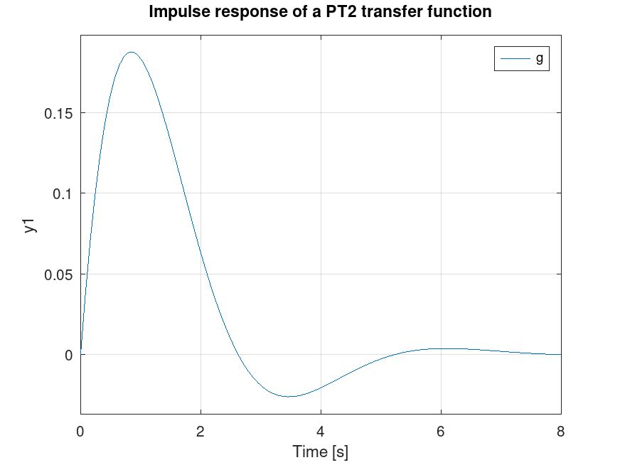
Demonstration 1
The following code
 clf;
 s = tf('s');
 g = 1/(2*s^2+3*s+4);
 impulse(g);
 title ("Impulse response of a PT2 transfer function");
Produces the following figure
| Figure 1 |
|---|
 |
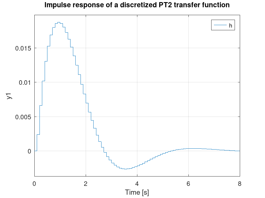
Demonstration 2
The following code
 clf;
 s = tf('s');
 g = 1/(2*s^2+3*s+4);
 h = c2d(g,0.1);
 impulse(h);
 title ("Impulse response of a discretized PT2 transfer function");
Produces the following figure
| Figure 1 |
|---|
 |
Package: control