Function Reference: lsim

Function File: lsim (sys, u)

Function File: lsim (sys1, sys2, …, sysN, u)

Function File: lsim (sys1, 'style1', …, sysN, 'styleN', u)

Function File: lsim (sys1, …, u, t)

Function File: lsim (sys1, …, u, t, x0)

Function File: [y, t, x] = lsim (sys, u)

Function File: [y, t, x] = lsim (sys, u, t)

Function File: [y, t, x] = lsim (sys, u, t, x0)

Simulate LTI model response to arbitrary inputs. If no output arguments are given, the system response is plotted on the screen.

Inputs

sys: LTI model. System must be proper, i.e. it must not have more zeros than poles.
u: Vector or array of input signal. Needs length(t) rows and as many columns as there are inputs. If sys is a single-input system, row vectors u of length length(t) are accepted as well.
t: Time vector. Should be evenly spaced. If sys is a continuous-time system and t is a real scalar, sys is discretized with sampling time tsam = t/(rows(u)-1). If sys is a discrete-time system and t is not specified, vector t is assumed to be 0 : tsam : tsam*(rows(u)-1).
x0: Vector of initial conditions for each state. If not specified, a zero vector is assumed.
’style’: Line style and color, e.g. ’r’ for a solid red line or ’-.k’ for a dash-dotted black line. See help plot for details.

Outputs

y: Output response array. Has as many rows as time samples (length of t) and as many columns as outputs.
t: Time row vector. It is always evenly spaced.
x: State trajectories array. Has length (t) rows and as many columns as states.

See also: impulse, initial, step.

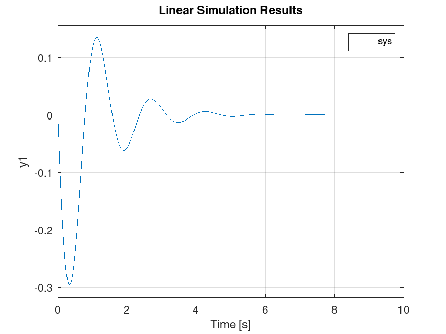
Demonstration 1

The following code

 clf;
 A = [-3   0   0;
       0  -2   1;
      10 -17   0];
 B = [4;
      0;
      0];
 C = [0 0 1];
 D = 0;
 sys = ss(A,B,C,D);
 t = 0:0.01:10;
 u = zeros (length(t) ,1);
 x0 = [0 0.1 0];
 lsim(sys, u, t, x0);

Produces the following figure

Figure 1

Package: control