
|
Octave-Forge - Extra packages for GNU Octave |
| Home · Packages · Developers · Documentation · FAQ · Bugs · Mailing Lists · Links · Code |
|
|
Octave-Forge - Extra packages for GNU Octave |
| Home · Packages · Developers · Documentation · FAQ · Bugs · Mailing Lists · Links · Code |
Function File: [yhat, lambda] = regdatasmooth (x, y, [options])
Smooths the y vs. x values of 1D data by Tikhonov regularization. The smooth y-values are returned as yhat. The regularization parameter lambda that was used for the smoothing may also be returned.
Note: the options have changed! Currently supported input options are (multiple options are allowed):
"d",value- the smoothing derivative to use (default = 2)
"lambda",value- the regularization paramater to use
"stdev",value- the standard deviation of the measurement of y; an optimal value for lambda will be determined by matching the provided value with the standard devation of yhat-y; if the option "relative" is also used, then a relative standard deviation is inferred
"gcv"- use generalized cross-validation to determine the optimal value for lambda; if neither "lambda" nor "stdev" options are given, this option is implied
"lguess",value- the initial value for lambda to use in the iterative minimization algorithm to find the optimal value (default = 1)
"xhat",vector- A vector of x-values to use for the smooth curve; must be monotonically increasing and must at least span the data
"weights",vector- A vector of weighting values for fitting each point in the data.
"relative"- use relative differences for the goodnes of fit term. Conflicts with the "weights" option.
"midpointrule"- use the midpoint rule for the integration terms rather than a direct sum; this option conflicts with the option "xhat"
Please run the demos for example usage.
References: Anal. Chem. (2003) 75, 3631; AIChE J. (2006) 52, 325
See also: rgdtsmcorewrap rgdtsmcore
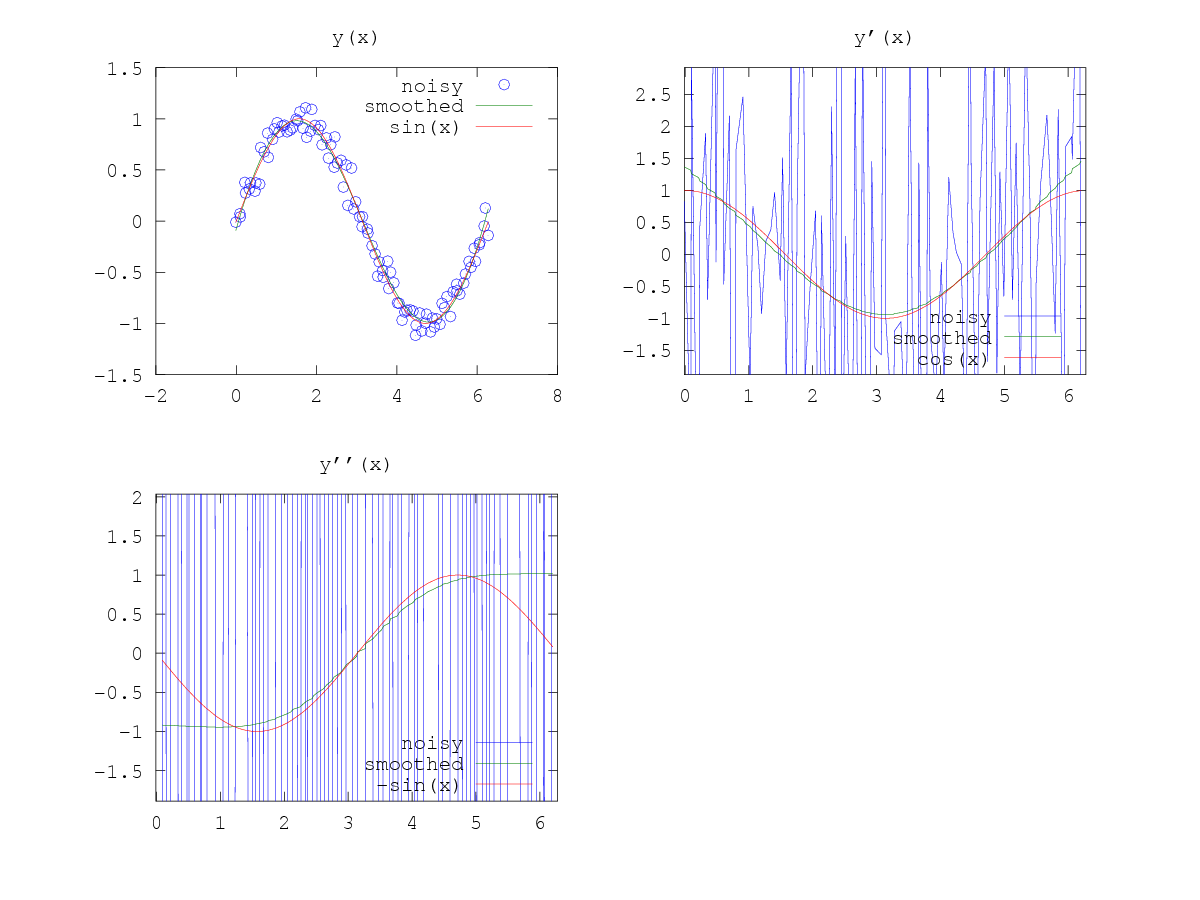
The following code
 npts = 100;
 x = linspace(0,2*pi,npts)';
 x = x + 2*pi/npts*(rand(npts,1)-0.5);
 y = sin(x);
 y = y + 1e-1*randn(npts,1);
 yp = ddmat(x,1)*y;
 y2p = ddmat(x,2)*y;
 [yh, lambda] = regdatasmooth (x, y, "d",4,"stdev",1e-1,"midpointrule");
 lambda
 yhp = ddmat(x,1)*yh;
 yh2p = ddmat(x,2)*yh;
 clf
 subplot(221)
 plot(x,y,'o','markersize',5,x,yh,x,sin(x))
 title("y(x)")
 legend("noisy","smoothed","sin(x)","location","northeast");
 subplot(222)
 plot(x(1:end-1),[yp,yhp,cos(x(1:end-1))])
 axis([min(x),max(x),min(yhp)-abs(min(yhp)),max(yhp)*2])
 title("y'(x)")
 legend("noisy","smoothed","cos(x)","location","southeast");
 subplot(223)
 plot(x(2:end-1),[y2p,yh2p,-sin(x(2:end-1))])
 axis([min(x),max(x),min(yh2p)-abs(min(yh2p)),max(yh2p)*2])
 title("y''(x)")
 legend("noisy","smoothed","-sin(x)","location","southeast");
 %--------------------------------------------------------
 % smoothing of monotonic data, using "stdev" to determine the optimal lambda
Produces the following output
lambda = 1
and the following figure
| Figure 1 |
|---|
 |
The following code
 npts = 20;
 x = rand(npts,1)*2*pi;
 y = sin(x);
 y = y + 1e-1*randn(npts,1);
 xh = linspace(0,2*pi,200)';
 [yh, lambda] = regdatasmooth (x, y, "d", 3, "xhat", xh);
 lambda
 clf
 figure(1);
 plot(x,y,'o','markersize',10,xh,yh,xh,sin(xh))
 title("y(x)")
 legend("noisy","smoothed","sin(x)","location","northeast");
 %--------------------------------------------------------
 % smoothing of scattered data, using "gcv" to determine the optimal lambda
Produces the following output
lambda = 0.0011140
and the following figure
| Figure 1 |
|---|
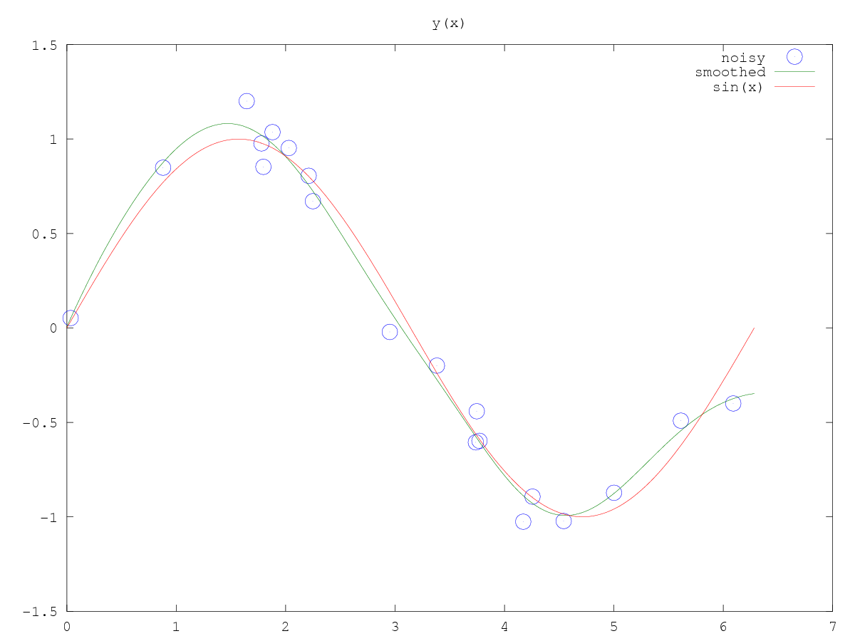 |
Package: data-smoothing