Function Reference: gaussmf

Function File: y = gaussmf (x, params)

Function File: y = gaussmf ([x1 x2 ... xn], [sig c])

For a given domain x and parameters params (or [sig c]), return the corresponding y values for the Gaussian membership function. This membership function is shaped like the Gaussian (normal) distribution, but scaled to have a maximum value of 1. By contrast, the area under the Gaussian distribution curve is 1.

The argument x must be a real number or a non-empty vector of strictly increasing real numbers, and sig and c must be real numbers. This membership function satisfies the equation:

f(x) = exp((-(x - c)^2)/(2 * sig^2))

which always returns values in the range [0, 1].

Just as for the Gaussian (normal) distribution, the parameters sig and c represent:

sig^2 == the variance (a measure of the width of the curve)
c == the center (the mean; the x value of the peak)

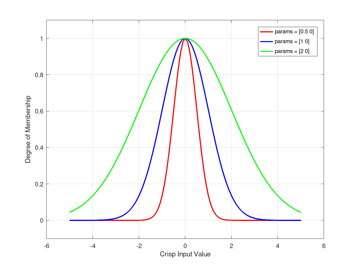
For larger values of sig, the curve is flatter, and for smaller values of sig, the curve is narrower. The y value at the center is always 1:

f(c) == 1

To run the demonstration code, type demo('gaussmf') at the Octave prompt.

See also: dsigmf, gauss2mf, gbellmf, pimf, psigmf, sigmf, smf, trapmf, trimf, zmf.

Demonstration 1

The following code

 x = -5:0.1:5;
 params = [0.5 0];
 y1 = gaussmf(x, params);
 params = [1 0];
 y2 = gaussmf(x, params);
 params = [2 0];
 y3 = gaussmf(x, params);
 figure('NumberTitle', 'off', 'Name', 'gaussmf demo');
 plot(x, y1, 'r;params = [0.5 0];', 'LineWidth', 2);
 hold on ;
 plot(x, y2, 'b;params = [1 0];', 'LineWidth', 2);
 hold on ;
 plot(x, y3, 'g;params = [2 0];', 'LineWidth', 2);
 ylim([-0.1 1.1]);
 xlabel('Crisp Input Value');
 ylabel('Degree of Membership');
 grid;
 hold;

Produces the following figure

Figure 1

Package: fuzzy-logic-toolkit