Function Reference: gustafson

Function File: cluster_centers = gustafson_kessel (input_data, num_clusters)

Function File: cluster_centers = gustafson_kessel (input_data, num_clusters, cluster_volume)

Function File: cluster_centers = gustafson_kessel (input_data, num_clusters, cluster_volume, options)

Function File: cluster_centers = gustafson_kessel (input_data, num_clusters, cluster_volume, [m, max_iterations, epsilon, display_intermediate_results])

Function File: [cluster_centers, soft_partition, obj_fcn_history] = gustafson_kessel (input_data, num_clusters)

Function File: [cluster_centers, soft_partition, obj_fcn_history] = gustafson_kessel (input_data, num_clusters, cluster_volume)

Function File: [cluster_centers, soft_partition, obj_fcn_history] = gustafson_kessel (input_data, num_clusters, cluster_volume, options)

Function File: [cluster_centers, soft_partition, obj_fcn_history] = gustafson_kessel (input_data, num_clusters, cluster_volume, [m, max_iterations, epsilon, display_intermediate_results])

Using the Gustafson-Kessel algorithm, calculate and return the soft partition of a set of unlabeled data points.

Also, if display_intermediate_results is true, display intermediate results after each iteration. Note that because the initial cluster prototypes are randomly selected locations in the ranges determined by the input data, the results of this function are nondeterministic.

The required arguments to gustafson_kessel are:

input_data - a matrix of input data points; each row corresponds to one point
num_clusters - the number of clusters to form

The third (optional) argument to gustafson_kessel is a vector of cluster volumes. If omitted, a vector of 1’s will be used as the default.

The fourth (optional) argument to gustafson_kessel is a vector consisting of:

m - the parameter (exponent) in the objective function; default = 2.0
max_iterations - the maximum number of iterations before stopping; default = 100
epsilon - the stopping criteria; default = 1e-5
display_intermediate_results - if 1, display results after each iteration, and if 0, do not; default = 1

The default values are used if any of the four elements of the vector are missing or evaluate to NaN.

The return values are:

cluster_centers - a matrix of the cluster centers; each row corresponds to one point
soft_partition - a constrained soft partition matrix
obj_fcn_history - the values of the objective function after each iteration

Three important matrices used in the calculation are X (the input points to be clustered), V (the cluster centers), and Mu (the membership of each data point in each cluster). Each row of X and V denotes a single point, and Mu(i, j) denotes the membership degree of input point X(j, :) in the cluster having center V(i, :).

X is identical to the required argument input_data; V is identical to the output cluster_centers; and Mu is identical to the output soft_partition.

If n denotes the number of input points and k denotes the number of clusters to be formed, then X, V, and Mu have the dimensions:

                              1    2   ...  #features
                         1 [                           ]
   X  =  input_data  =   2 [                           ]
                       ... [                           ]
                         n [                           ]

                                   1    2   ...  #features
                              1 [                           ]
   V  =  cluster_centers  =   2 [                           ]
                            ... [                           ]
                              k [                           ]

                                   1    2   ...   n
                              1 [                    ]
   Mu  =  soft_partition  =   2 [                    ]
                            ... [                    ]
                              k [                    ]

See also: fcm, partition_coeff, partition_entropy, xie_beni_index.

Demonstration 1

The following code

 ## This demo:
 ##    - classifies a small set of unlabeled data points using
 ##      the Gustafson-Kessel algorithm into two fuzzy clusters
 ##    - plots the input points together with the cluster centers
 ##    - evaluates the quality of the resulting clusters using
 ##      three validity measures: the partition coefficient, the
 ##      partition entropy, and the Xie-Beni validity index
 ##
 ## Note: The input_data is taken from Chapter 13, Example 17 in
 ##       Fuzzy Logic: Intelligence, Control and Information, by
 ##       J. Yen and R. Langari, Prentice Hall, 1999, page 381
 ##       (International Edition). 
 
 ## Use gustafson_kessel to classify the input_data.
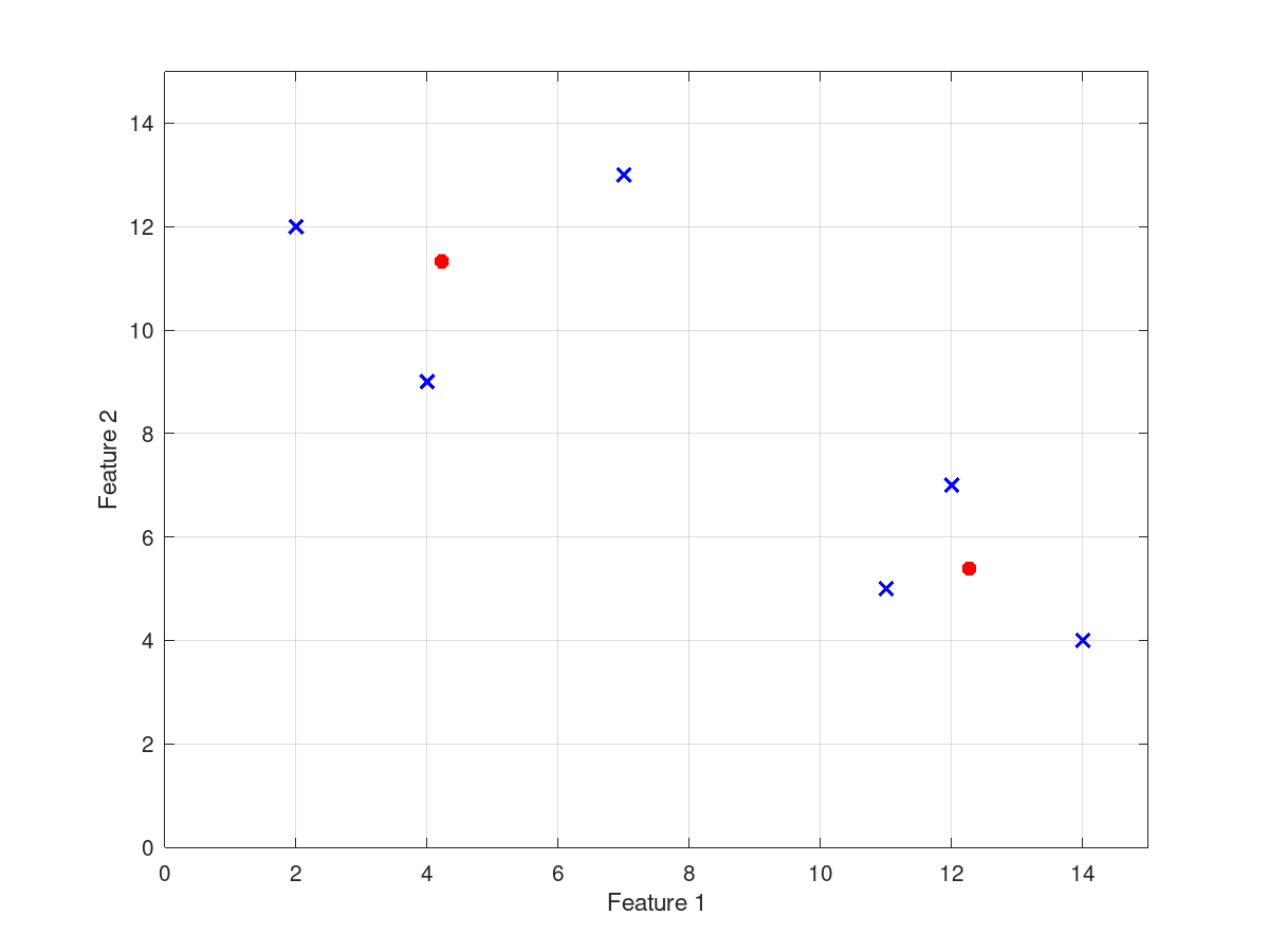
 input_data = [2 12; 4 9; 7 13; 11 5; 12 7; 14 4];
 number_of_clusters = 2;
 [cluster_centers, soft_partition, obj_fcn_history] = ...
   gustafson_kessel (input_data, number_of_clusters)
 
 ## Plot the data points as small blue x's.
 figure ('NumberTitle', 'off', 'Name', 'Gustafson-Kessel Demo 1');
 for i = 1 : rows (input_data)
   plot (input_data(i, 1), input_data(i, 2), 'LineWidth', 2, ...
         'marker', 'x', 'color', 'b');
   hold on;
 endfor
 
 ## Plot the cluster centers as larger red *'s.
 for i = 1 : number_of_clusters
   plot (cluster_centers(i, 1), cluster_centers(i, 2), ...
         'LineWidth', 4, 'marker', '*', 'color', 'r');
   hold on;
 endfor
 
 ## Make the figure look a little better:
 ##    - scale and label the axes
 ##    - show gridlines
 xlim ([0 15]);
 ylim ([0 15]);
 xlabel ('Feature 1');
 ylabel ('Feature 2');
 grid
 hold
 
 ## Calculate and print the three validity measures.
 printf ("Partition Coefficient: %f\n", ...
         partition_coeff (soft_partition));
 printf ("Partition Entropy (with a = 2): %f\n", ...
         partition_entropy (soft_partition, 2));
 printf ("Xie-Beni Index: %f\n\n", ...
         xie_beni_index (input_data, cluster_centers, ...
         soft_partition));

Produces the following output

Iteration count = 1,  Objective fcn = 56.699686
Iteration count = 2,  Objective fcn = 45.237089
Iteration count = 3,  Objective fcn = 38.430648
Iteration count = 4,  Objective fcn = 34.623038
Iteration count = 5,  Objective fcn = 31.224824
Iteration count = 6,  Objective fcn = 28.356924
Iteration count = 7,  Objective fcn = 27.395198
Iteration count = 8,  Objective fcn = 26.912511
Iteration count = 9,  Objective fcn = 26.440829
Iteration count = 10,  Objective fcn = 26.048048
Iteration count = 11,  Objective fcn = 25.809495
Iteration count = 12,  Objective fcn = 25.702798
Iteration count = 13,  Objective fcn = 25.663973
Iteration count = 14,  Objective fcn = 25.651023
Iteration count = 15,  Objective fcn = 25.646767
Iteration count = 16,  Objective fcn = 25.645357
Iteration count = 17,  Objective fcn = 25.644885
Iteration count = 18,  Objective fcn = 25.644726
Iteration count = 19,  Objective fcn = 25.644672
Iteration count = 20,  Objective fcn = 25.644653
Iteration count = 21,  Objective fcn = 25.644647
Iteration count = 22,  Objective fcn = 25.644645
Iteration count = 23,  Objective fcn = 25.644644
Iteration count = 24,  Objective fcn = 25.644644
Iteration count = 25,  Objective fcn = 25.644644
Iteration count = 26,  Objective fcn = 25.644644
Iteration count = 27,  Objective fcn = 25.644644
Iteration count = 28,  Objective fcn = 25.644644
Iteration count = 29,  Objective fcn = 25.644644
Iteration count = 30,  Objective fcn = 25.644644
cluster_centers =

    4.2228   11.3276
   12.2661    5.3877

soft_partition =

   0.934026   0.890524   0.870505   0.023529   0.028088   0.012592
   0.065974   0.109476   0.129495   0.976471   0.971912   0.987408

obj_fcn_history =

 Columns 1 through 8:

   56.700   45.237   38.431   34.623   31.225   28.357   27.395   26.913

 Columns 9 through 16:

   26.441   26.048   25.809   25.703   25.664   25.651   25.647   25.645

 Columns 17 through 24:

   25.645   25.645   25.645   25.645   25.645   25.645   25.645   25.645

 Columns 25 through 30:

   25.645   25.645   25.645   25.645   25.645   25.645

Partition Coefficient: 0.888484
Partition Entropy (with a = 2): 0.308027
Xie-Beni Index: 0.107028

and the following figure

Figure 1

Demonstration 2

The following code

 ## This demo:
 ##    - classifies three-dimensional unlabeled data points using
 ##      the Gustafson-Kessel algorithm into three fuzzy clusters
 ##    - plots the input points together with the cluster centers
 ##    - evaluates the quality of the resulting clusters using
 ##      three validity measures: the partition coefficient, the
 ##      partition entropy, and the Xie-Beni validity index
 ##
 ## Note: The input_data was selected to form three areas of
 ##       different shapes.
 
 ## Use gustafson_kessel to classify the input_data.
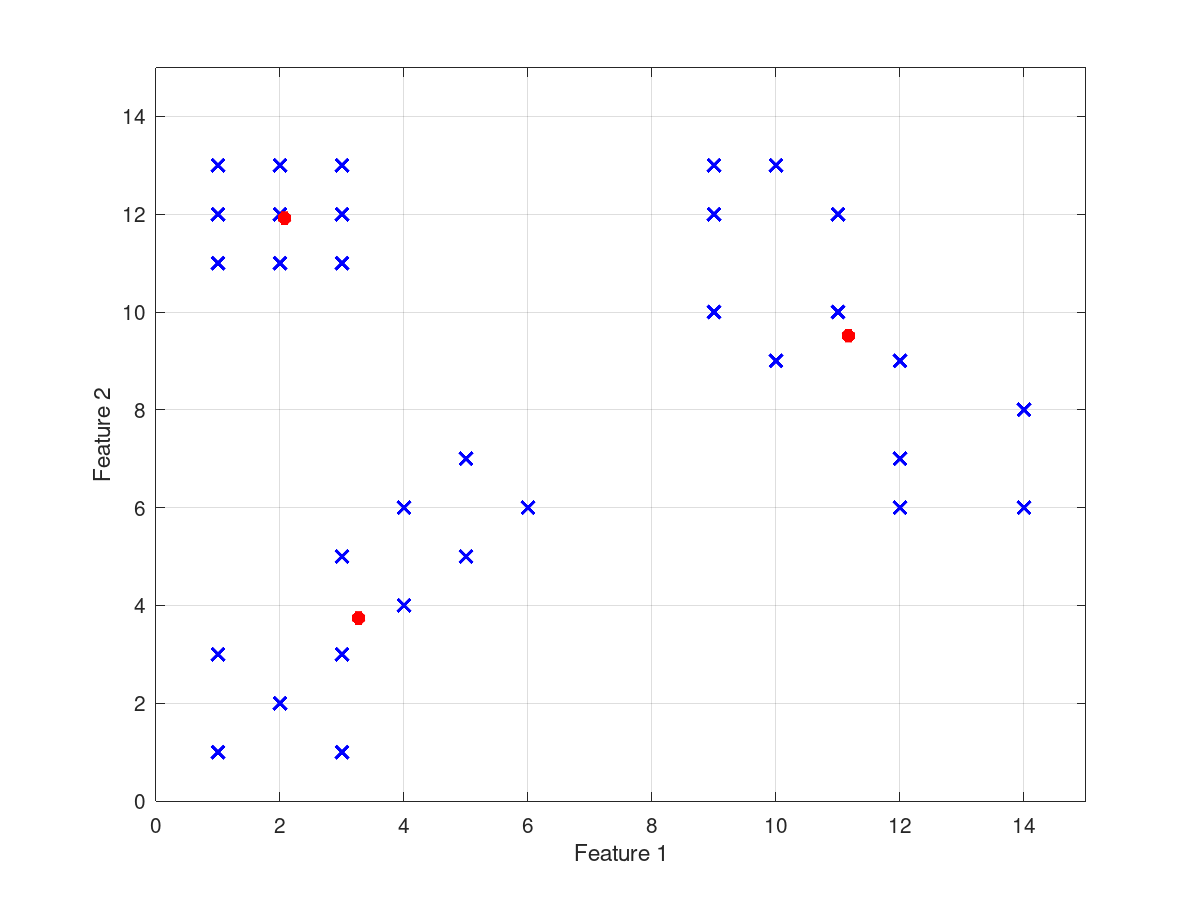
 input_data = [1 11 5; 1 12 6; 1 13 5; 2 11 7; 2 12 6; 2 13 7;
               3 11 6; 3 12 5; 3 13 7; 1 1 10; 1 3 9; 2 2 11;
               3 1 9; 3 3 10; 3 5 11; 4 4 9; 4 6 8; 5 5 8; 5 7 9;
               6 6 10; 9 10 12; 9 12 13; 9 13 14; 10 9 13; 10 13 12;
               11 10 14; 11 12 13; 12 6 12; 12 7 15; 12 9 15;
               14 6 14; 14 8 13];
 number_of_clusters = 3;
 [cluster_centers, soft_partition, obj_fcn_history] = ...
   gustafson_kessel (input_data, number_of_clusters, [1 1 1], ...
                     [NaN NaN NaN 0])
 
 ## Plot the data points in two dimensions (using features 1 & 2)
 ## as small blue x's.
 figure ('NumberTitle', 'off', 'Name', 'Gustafson-Kessel Demo 2');
 for i = 1 : rows (input_data)
   plot (input_data(i, 1), input_data(i, 2), 'LineWidth', 2, ...
         'marker', 'x', 'color', 'b');
   hold on;
 endfor
 
 ## Plot the cluster centers in two dimensions
 ## (using features 1 & 2) as larger red *'s.
 for i = 1 : number_of_clusters
   plot (cluster_centers(i, 1), cluster_centers(i, 2), ...
         'LineWidth', 4, 'marker', '*', 'color', 'r');
   hold on;
 endfor
 
 ## Make the figure look a little better:
 ##    - scale and label the axes
 ##    - show gridlines
 xlim ([0 15]);
 ylim ([0 15]);
 xlabel ('Feature 1');
 ylabel ('Feature 2');
 grid
  
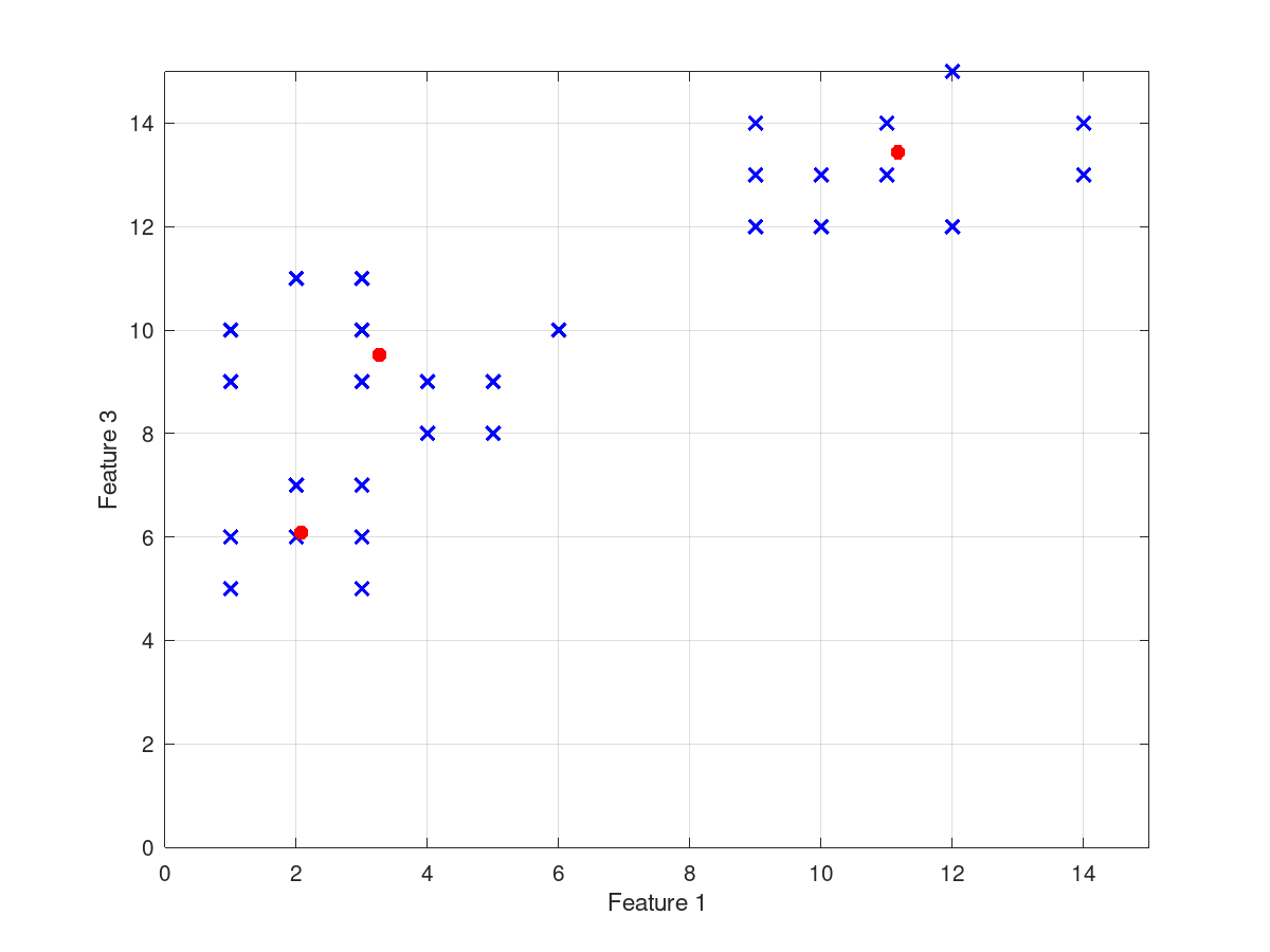
 ## Plot the data points in two dimensions
 ## (using features 1 & 3) as small blue x's.
 figure ('NumberTitle', 'off', 'Name', 'Gustafson-Kessel Demo 2');
 for i = 1 : rows (input_data)
   plot (input_data(i, 1), input_data(i, 3), 'LineWidth', 2, ...
         'marker', 'x', 'color', 'b');
   hold on;
 endfor
 
 ## Plot the cluster centers in two dimensions
 ## (using features 1 & 3) as larger red *'s.
 for i = 1 : number_of_clusters
   plot (cluster_centers(i, 1), cluster_centers(i, 3), ...
         'LineWidth', 4, 'marker', '*', 'color', 'r');
   hold on;
 endfor
 
 ## Make the figure look a little better:
 ##    - scale and label the axes
 ##    - show gridlines
 xlim ([0 15]);
 ylim ([0 15]);
 xlabel ('Feature 1');
 ylabel ('Feature 3');
 grid
 hold
 
 ## Calculate and print the three validity measures.
 printf ("Partition Coefficient: %f\n", ...
         partition_coeff (soft_partition));
 printf ("Partition Entropy (with a = 2): %f\n", ...
         partition_entropy (soft_partition, 2));
 printf ("Xie-Beni Index: %f\n\n", ...
         xie_beni_index (input_data, cluster_centers, ...
         soft_partition));

Produces the following output

cluster_centers =

   11.1675    9.5123   13.4360
    2.0744   11.9210    6.0810
    3.2679    3.7416    9.5189

soft_partition =

 Columns 1 through 5:

   0.011156940   0.007168151   0.009256966   0.013793209   0.000061636
   0.969713610   0.983129646   0.980099574   0.961231963   0.999849093
   0.019129450   0.009702203   0.010643461   0.024974828   0.000089272

 Columns 6 through 10:

   0.018522392   0.010694147   0.025263997   0.020998218   0.009263487
   0.961740379   0.967527444   0.933398914   0.955321662   0.022954702
   0.019737230   0.021778409   0.041337089   0.023680120   0.967781811

 Columns 11 through 15:

   0.018978727   0.013116906   0.022733658   0.002488192   0.031043587
   0.061140856   0.029744554   0.056773300   0.006522152   0.079764432
   0.919880417   0.957138541   0.920493042   0.990989656   0.889191981

 Columns 16 through 20:

   0.004486762   0.029447624   0.026948323   0.033445437   0.054461524
   0.013944143   0.149981735   0.096878351   0.143129341   0.127672201
   0.981569094   0.820570641   0.876173326   0.823425222   0.817866275

 Columns 21 through 25:

   0.729602066   0.902079011   0.863380551   0.899998020   0.781772579
   0.132307043   0.053108509   0.076957490   0.052617552   0.108651912
   0.138090890   0.044812480   0.059661959   0.047384429   0.109575510

 Columns 26 through 30:

   0.980412577   0.887353560   0.817815530   0.895170165   0.921166920
   0.010973086   0.058410139   0.100649182   0.063517883   0.046917106
   0.008614337   0.054236301   0.081535289   0.041311952   0.031915974

 Columns 31 and 32:

   0.931435604   0.874466392
   0.042583126   0.072534103
   0.025981271   0.052999504

obj_fcn_history =

 Columns 1 through 8:

   243.86   184.80   158.32   140.91   130.79   125.97   123.46   121.81

 Columns 9 through 16:

   120.82   120.34   120.15   120.08   120.05   120.04   120.04   120.03

 Columns 17 through 24:

   120.03   120.03   120.03   120.03   120.03   120.03   120.03   120.03

 Columns 25 through 29:

   120.03   120.03   120.03   120.03   120.03

Partition Coefficient: 0.841843
Partition Entropy (with a = 2): 0.472418
Xie-Beni Index: 0.192631

and the following figures

Figure 1	Figure 2

Package: fuzzy-logic-toolkit