- Function File: cauchy
(N, r, x, f )¶ Return the Taylor coefficients and numerical differentiation of a function.
f for the first N-1 coefficients or derivatives using the fft.
N is the number of points to evaluate,
r is the radius of convergence, needs to be chosen less then the smallest singularity,
x is point to evaluate the Taylor expansion or differentiation. For example,If x is a scalar, the function f is evaluated in a row vector of length N. If x is a column vector, f is evaluated in a matrix of length(x)-by-N elements and must return a matrix of the same size.
d = cauchy(16, 1.5, 0, @(x) exp(x));
d(2) = 1.0000 # first (2-1) derivative of function f (index starts from zero)
Demonstration 1
The following code
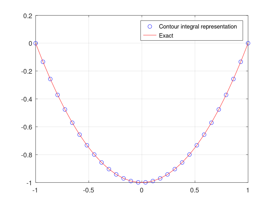
 # Cauchy integral formula: Application to Hermite polynomials
 # Author: Fernando Damian Nieuwveldt
 # Edited by: Juan Pablo Carbajal

 Hnx     = @(t,x) exp ( bsxfun (@minus, kron(t(:).', x(:)) , t(:).'.^2/2) );
 hermite = @(order,x) cauchy(32, 0.5, 0, @(t)Hnx(t,x))(:, order+1);

 t    = linspace(-1,1,30);
 he2  = hermite(2,t);
 he2_ = t.^2-1;

 figure(1)
 clf
 plot(t,he2,'bo;Contour integral representation;', t,he2_,'r;Exact;');
 grid

 % --------------------------------------------------------------------------
 % The plots compares the approximation of the Hermite polynomial using the
 % Cauchy integral (circles) and the corresposind polynomial H_2(x) = x.^2 - 1.
 % See http://en.wikipedia.org/wiki/Hermite_polynomials#Contour_integral_representation
Produces the following figure
| Figure 1 |
|---|
 |
Demonstration 2
The following code
# Cauchy integral formula: Application to Hermite polynomials
# Author: Fernando Damian Nieuwveldt
# Edited by: Juan Pablo Carbajal
xx = sort (rand (100,1));
yy = sin (3*2*pi*xx);
# Exact first derivative derivative
diffy = 6*pi*cos (3*2*pi*xx);
np = [10 15 30 100];
for i =1:4
idx = sort(randperm (100,np(i)));
x = xx(idx);
y = yy(idx);
p = spline (x,y);
yval = ppval (ppder(p),x);
# Use the cauchy formula for computing the derivatives
deriv = cauchy (fix (np(i)/4), .1, x, @(x) sin (3*2*pi*x));
subplot(2,2,i)
h = plot(xx,diffy,'-b;Exact;',...
x,yval,'-or;ppder solution;',...
x,deriv(:,2),'-og;Cauchy formula;');
set(h(1),'linewidth',2);
set(h(2:3),'markersize',3);
legend(h, 'Location','Northoutside','Orientation','horizontal');
if i!=1
legend('hide');
end
end
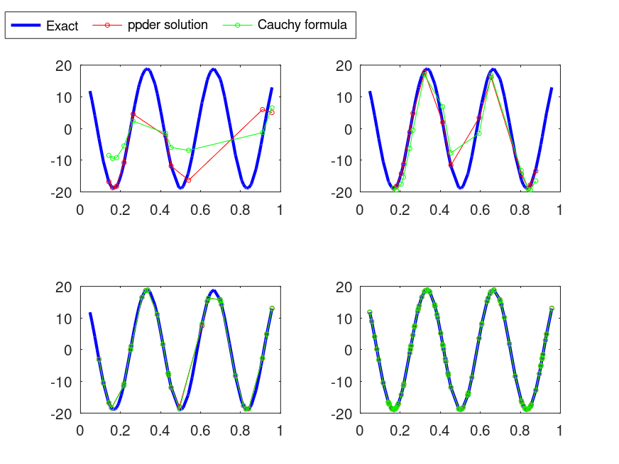
% --------------------------------------------------------------------------
% The plots compares the derivatives calculated with Cauchy and with ppder.
% Each subplot shows the results with increasing number of samples.
Produces the following figure
| Figure 1 |
|---|
 |
Package: general