Method on @infsup: X = fsolve (F)

Method on @infsup: X = fsolve (F, X0)

Method on @infsup: X = fsolve (F, X0, Y)

Method on @infsup: X = fsolve (…, OPTIONS)

Method on @infsup: [X, X_PAVING, X_INNER_IDX] = fsolve (…)

Compute the preimage of the set Y under function F.

Parameter Y is optional and without it solve F(x) = 0 for x ∈ X0. Without a starting box X0 the function is assumed to be univariate and the solution is searched among all real numbers.

The function must be an interval arithmetic function and may be multivariate, that is, X0 and Y may be vectors or arrays of intervals. The computational complexity largely depends on the dimension of X0.

Return value X is an interval enclosure of {x ∈ X0 |F(x) ∈ Y}. The optional return value X_PAVING is a matrix of non-overlapping interval values for x in each column, which form a more detailed enclosure for the preimage of Y. An index vector X_INNER_IDX indicates the columns of X_PAVING, which are guaranteed to be subsets of the preimage of Y.

This function uses the set inversion via interval arithmetic (SIVIA) algorithm. That is, X is bisected until F(X) is either a subset of Y or until they are disjoint.

fsolve (@cos, infsup(0, "pi"))
  ⇒ ans ⊂ [1.5646, 1.5708]

It is possible to use the following optimization options: MaxFunEvals, MaxIter, TolFun, TolX, Vectorize, Contract.

If Vectorize is true, the function F will be called with input arguments x(1), x(2), …, x(numel (X0)) and each input argument will carry a vector of different values which shall be computed simultaneously. If Y is a scalar or vector, Vectorize defaults to true. If Vectorize is false, the function F will receive only one input argument x at a time, which has the size of X0.

# Solve x1 ^ 2 + x2 ^ 2 = 1 for -3 ≤ x1, x2 ≤ 3,
# the exact solution is a unit circle
x = fsolve (@(x1, x2) x1.^2 + x2.^2, infsup ([-3; -3], [3; 3]), 1)
  ⇒ x ⊂ 2×1 interval vector

        [-1.002, +1.002]
      [-1.0079, +1.0079]

If Contract is true, the function F will be called with Y as an additional leading input argument and, in addition to the function value, must return a contraction of its input argument(s). A contraction for input argument x is a subset of x which contains all possible solutions for the equation F (x) = Y. Contractions can be computed using interval reverse operations, for example with @infsup/absrev which contracts the input argument for the absolute value function.

# Solve x1 ^ 2 + x2 ^ 2 = 1 for -3 ≤ x1, x2 ≤ 3 again,
# but now contractions speed up the algorithm.
function [fval, cx1, cx2] = f (y, x1, x2)
  # Forward evaluation
  x1_sqr = x1 .^ 2;
  x2_sqr = x2 .^ 2;
  fval = x1_sqr + x2_sqr;

  # Reverse evaluation and contraction
  y = intersect (y, fval);
  # Contract the squares
  x1_sqr = intersect (x1_sqr, y - x2_sqr);
  x2_sqr = intersect (x2_sqr, y - x1_sqr);
  # Contract the parameters
  cx1 = sqrrev (x1_sqr, x1);
  cx2 = sqrrev (x2_sqr, x2);
endfunction

x = fsolve (@f, infsup ([-3; -3], [3; 3]), 1, ...
            struct ('Contract', true))
  ⇒ x = 2×1 interval vector

      [-1, +1]
      [-1, +1]

It is possible to combine options Vectorize and Contract. Depending on the combination, function F should have one of the following signatures.

function fval = f (x)

Vectorize = false and Contract = false.

function fval = f (x1, x2, …, xN)

Vectorize = true and Contract = false.

function [fval, cx] = f (y, x)

Vectorize = false and Contract = true. cx is a contraction of x.

function [fval, cx1, cx2, …, cxN] = f (y, x1, x2, …, xN)

Vectorize = true and Contract = true. cx1 is a contraction of x1, cx2 is a contraction of x2, and so on.

Note on performance: The bisection method is a brute-force approach to exhaust the function’s domain and requires a lot of function evaluations. It is highly recommended to use a function F which allows vectorization. For higher dimensions of X0 it is also necessary to use a contraction function.

Accuracy: The result is a valid enclosure.

See also: @infsup/fzero, ctc_union, ctc_intersect, optimset.

Demonstration 1

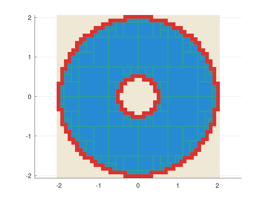Demonstration 2

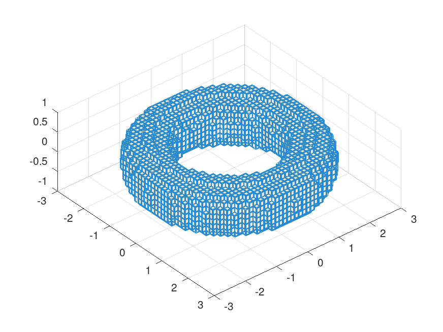Package: interval