|
Octave-Forge - Extra packages for GNU Octave |
| Home · Packages · Developers · Documentation · FAQ · Bugs · Mailing Lists · Links · Code |
fyp = irsa_dft (xp, yp, fxp, [lm])
Compute Discrete Fourier Transformations of irregular sampled time series
[xp,yp]using dft(f) = sum_(k=1)^Nyp[k] * exp(-2*pi*I*xp[k]*f)for every f in fxpInput:
xp : Columnvector – sampling points
yp : Matrix with the timeseries values in its columns
fxp : Vector – frequency points for the DFT
lm : Boolean – use lesser memory if 'true' (slower). Default is 'false'.
Output:
fyp : Matrix with values of the DFTs in its columns
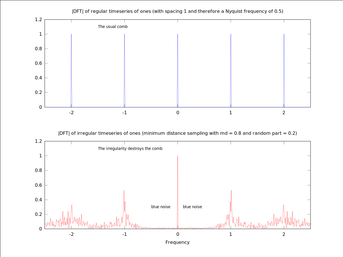
The following code
 N = 100;
 eqxp = [0:1:N-1].';
 mdxp = irsa_mdsp( .8 , .2, N, "randn" );
 yp = ones(N,1);
 hifac = 5; ofac = 1;
 eqfxp = irsa_dftfp( eqxp, hifac, ofac );
 eqfyp = irsa_dft( eqxp, yp, eqfxp );
 [eqfxp,idx] = sort( eqfxp ); eqfyp = eqfyp(idx);
 ## Plot
 figure();
 subplot( 211 )
 plot( eqfxp, abs(eqfyp)/N, '-b' ); text();
 title( "|DFT| of regular timeseries of ones (with spacing 1 and therefore a Nyquist frequency of 0.5)" );
 text( -1.5, 1.1, "The usual comb" );
 axis([-2.5,2.5,0,1.2]);
 legend('off');
 mdfxp = irsa_dftfp( mdxp, hifac, ofac );
 mdfyp = irsa_dft( mdxp, yp, mdfxp );
 [mdfxp,idx] = sort( mdfxp ); mdfyp = mdfyp(idx);
 subplot( 212 )
 plot( mdfxp, abs(mdfyp)/N, '-r' ); text();
 title( "|DFT| of irregular timeseries of ones (minimum distance sampling with md = 0.8 and random part = 0.2)" );
 text( -1.5, 1.1, "The irregularity destroys the comb" );
 text( -0.5,0.3,"blue noise"); text( 0.1,0.3,"blue noise" );
 xlabel( "Frequency" );
 axis([-2.5,2.5,0,1.2]);
 legend('off');
Produces the following figure
| Figure 1 |
|---|
 |