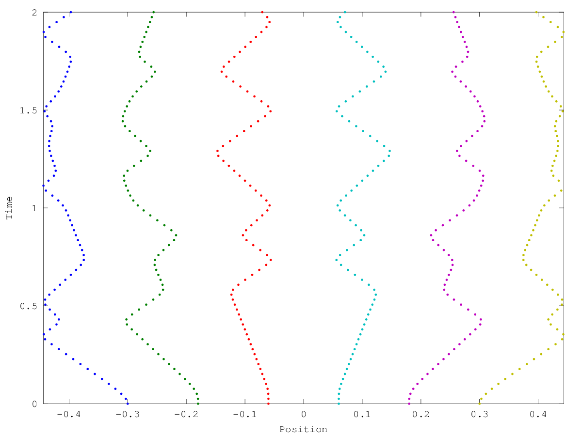
The following code

 N       = 6;
 P0      = linspace (-0.5+1/(N-1), 0.5-1/(N-1), N).';
 V0      = zeros (N, 1);
 nT      = 80;
 tspan   = linspace(0, 2, nT);
 [t P V] = mdsim ('demofunc1', tspan, P0, V0,'timestep',1e-3);

 figure (1)
 plot (P.',t,'.');
 xlabel ("Position")
 ylabel ("Time")
 axis tight

 disp("Initial values")
 disp ( sum ([V(:,1) P(:,1)], 1) )
 disp("Final values")
 disp ( sum ([V(:,end) P(:,end)], 1) )

 %-------------------------------------------------------------------
 % 1D particles with Lennard-Jones potential and periodic boundaries.
 % Velocity and position of the center of mass are conserved. 

Produces the following output

Initial values
   0.0000e+00  -5.5511e-17
Final values
   3.8858e-15   3.4417e-15

and the following figure

Figure 1

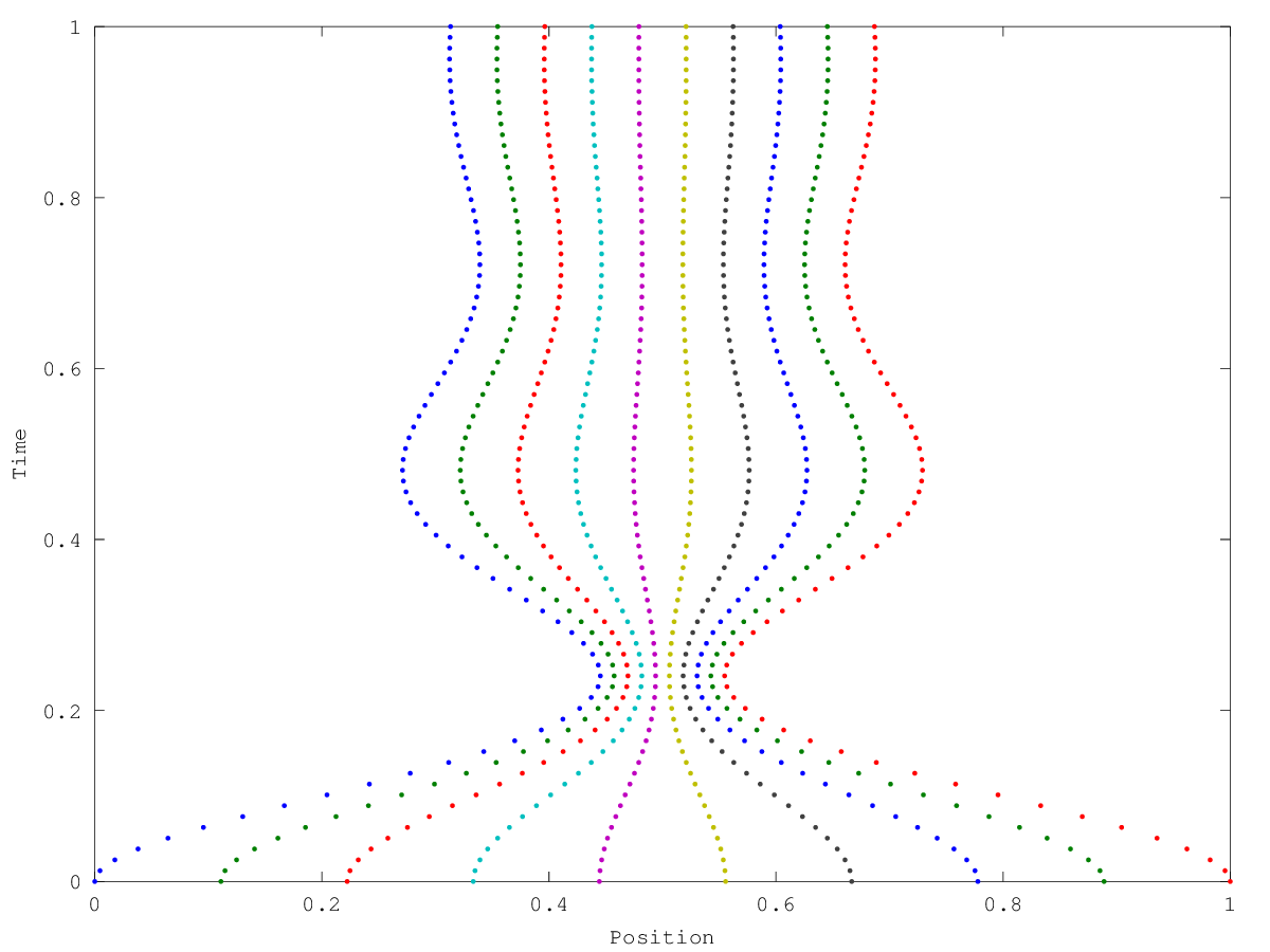
The following code

 N     = 10;
 P0    = linspace (0,1,N).';
 V0    = zeros (N, 1);
 nT    = 80;
 tspan = linspace(0, 1, nT);
 [t P] = mdsim ('demofunc2', tspan, P0, V0,'nonperiodic', true);

 figure (1)
 plot (P.',t,'.');
 xlabel ("Position")
 ylabel ("Time")

 %-------------------------------------------------------------------
 % 1D array of springs with damping proportional to relative velocity and
 % nonzero rest length.

Produces the following figure

Initial values
   0.0000e+00  -5.5511e-17
Final values
   3.8858e-15   3.4417e-15

and the following figure

Figure 1

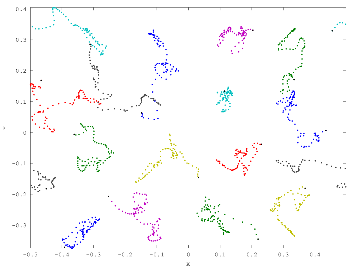
The following code

 
 input("NOTE: It may take a while.\nPress Ctrl-C to cancel or  to continue: ","s");

 N       = 4;
 [Px Py] = meshgrid (linspace (-0.5+0.5/(N-1), 0.5-0.5/(N-1), N));
 P0      = [Px(:) Py(:)];
 N       = size(P0,1);
 P0      = P0 + 0.1* 0.5/N *(2*rand (size (P0)) - 1);
 V0      = zeros (N, 2);
 nT      = 80;
 tspan   = linspace(0, 1, nT);
 [t P]   = mdsim ('demofunc3', tspan, P0, V0);
 x       = squeeze(P(:,1,:)); 
 y       = squeeze(P(:,2,:));

 figure (1)
 plot (x.',y.','.',x(:,end),y(:,end),'.k');
 xlabel ("X")
 ylabel ("Y")
 axis tight

 %-------------------------------------------------------------------
 % 2D particles with Lennard-Jones potential and periodic boundaries

Produces the following output

NOTE: It may take a while.
Press Ctrl-C to cancel or  to continue:

and the following figure

Figure 1