 NRBMAK: Construct the NURBS structure given the control points
            and the knots.

 Calling Sequence:

   nurbs   = nrbmak(cntrl,knots,[normalize]);

 INPUT:

   cntrl       : Control points, these can be either Cartesian or
 		homogeneous coordinates.

 		For a curve the control points are represented by a
 		matrix of size (dim,nu), for a surface a multidimensional
 		array of size (dim,nu,nv), for a volume a multidimensional array
 		of size (dim,nu,nv,nw). Where nu is number of points along
 		the parametric U direction, nv the number of points along
 		the V direction and nw the number of points along the W direction.
 		dim is the dimension. Valid options
 		are
 		2 .... (x,y)        2D Cartesian coordinates
 		3 .... (x,y,z)      3D Cartesian coordinates
 		4 .... (wx,wy,wz,w) 4D homogeneous coordinates

   knots	: Non-decreasing knot sequence spanning the interval
               [0.0,1.0]. It's assumed that the geometric entities
               are clamped to the start and end control points by knot
               multiplicities equal to the spline order (open knot vector).
               For curve knots form a vector and for surfaces (volumes)
               the knots are stored by two (three) vectors for U and V (and W)
               in a cell structure {uknots vknots} ({uknots vknots wknots}).

   normalize: if true, the knot vector is normalized to the interval [0, 1].
               Default value is false.

 OUTPUT:

   nurbs 	: Data structure for representing a NURBS entity

 NURBS Structure:

   Both curves and surfaces are represented by a structure that is
   compatible with the Spline Toolbox from Mathworks

 	nurbs.form   .... Type name 'B-NURBS'
 	nurbs.dim    .... Dimension of the control points
 	nurbs.number .... Number of Control points
       nurbs.coefs  .... Control Points
       nurbs.order  .... Order of the spline
       nurbs.knots  .... Knot sequence

   Note: the control points are always converted and stored within the
   NURBS structure as 4D homogeneous coordinates. A curve is always stored
   along the U direction, and the vknots element is an empty matrix. For
   a surface the spline order is a vector [du,dv] containing the order
   along the U and V directions respectively. For a volume the order is
   a vector [du dv dw]. Recall that order = degree + 1.

 Description:

   This function is used as a convenient means of constructing the NURBS
   data structure. Many of the other functions in the toolbox rely on the
   NURBS structure been correctly defined as shown above. The nrbmak not
   only constructs the proper structure, but also checks for consistency.
   The user is still free to build his own structure, in fact a few
   functions in the toolbox do this for convenience.

 Examples:

   Construct a 2D line from (0.0,0.0) to (1.5,3.0).
   For a straight line a spline of order 2 is required.
   Note that the knot sequence has a multiplicity of 2 at the
   start (0.0,0.0) and end (1.0 1.0) in order to clamp the ends.

   line = nrbmak([0.0 1.5; 0.0 3.0],[0.0 0.0 1.0 1.0]);
   nrbplot(line, 2);

   Construct a surface in the x-y plane i.e

     ^  (0.0,1.0) ------------ (1.0,1.0)
     |      |                      |
     | V    |                      |
     |      |      Surface         |
     |      |                      |
     |      |                      |
     |  (0.0,0.0) ------------ (1.0,0.0)
     |
     |------------------------------------>
                                       U

   coefs = cat(3,[0 0; 0 1],[1 1; 0 1]);
   knots = {[0 0 1 1]  [0 0 1 1]}
   plane = nrbmak(coefs,knots);
   nrbplot(plane, [2 2]);

    Copyright (C) 2000 Mark Spink, 2010-2018 Rafael Vazquez

    This program is free software: you can redistribute it and/or modify
    it under the terms of the GNU General Public License as published by
    the Free Software Foundation, either version 3 of the License, or
    (at your option) any later version.
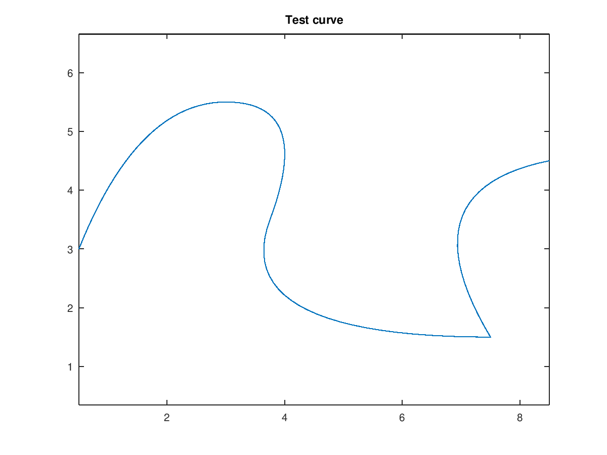
Demonstration 1
The following code
 pnts = [0.5 1.5 4.5 3.0 7.5 6.0 8.5;
         3.0 5.5 5.5 1.5 1.5 4.0 4.5;
         0.0 0.0 0.0 0.0 0.0 0.0 0.0];
 crv = nrbmak(pnts,[0 0 0 1/4 1/2 3/4 3/4 1 1 1]);
 nrbplot(crv,100)
 title('Test curve')
 hold off
Produces the following figure
| Figure 1 |
|---|
 |
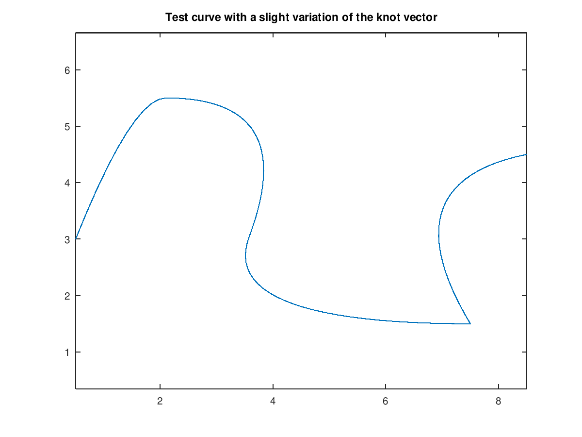
Demonstration 2
The following code
 pnts = [0.5 1.5 4.5 3.0 7.5 6.0 8.5;
         3.0 5.5 5.5 1.5 1.5 4.0 4.5;
         0.0 0.0 0.0 0.0 0.0 0.0 0.0];
 crv = nrbmak(pnts,[0 0 0 0.1 1/2 3/4 3/4 1 1 1]);
 nrbplot(crv,100)
 title('Test curve with a slight variation of the knot vector')
 hold off
Produces the following figure
| Figure 1 |
|---|
 |
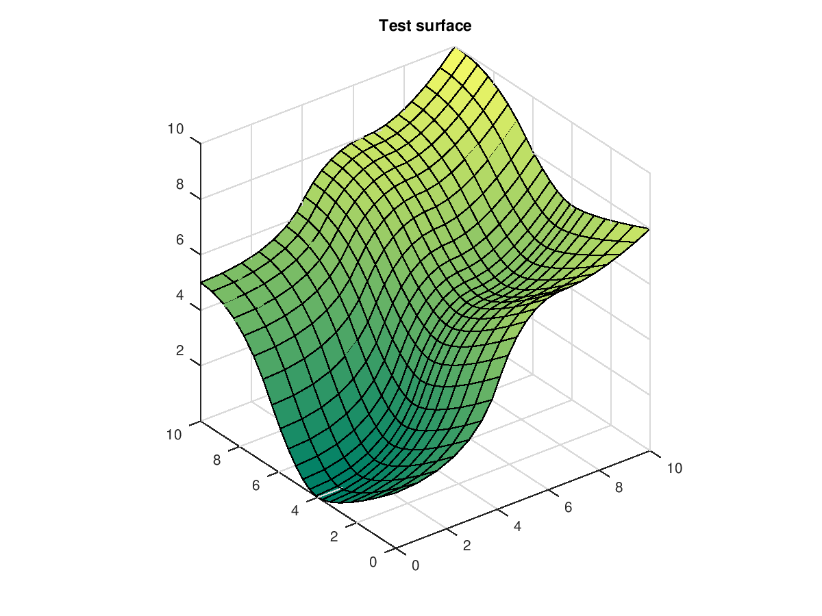
Demonstration 3
The following code
 pnts = zeros(3,5,5);
 pnts(:,:,1) = [ 0.0  3.0  5.0  8.0 10.0;
                 0.0  0.0  0.0  0.0  0.0;
                 2.0  2.0  7.0  7.0  8.0];
 pnts(:,:,2) = [ 0.0  3.0  5.0  8.0 10.0;
                 3.0  3.0  3.0  3.0  3.0;
                 0.0  0.0  5.0  5.0  7.0];
 pnts(:,:,3) = [ 0.0  3.0  5.0  8.0 10.0;
                 5.0  5.0  5.0  5.0  5.0;
                 0.0  0.0  5.0  5.0  7.0];
 pnts(:,:,4) = [ 0.0  3.0  5.0  8.0 10.0;
                 8.0  8.0  8.0  8.0  8.0;
                 5.0  5.0  8.0  8.0 10.0];
 pnts(:,:,5) = [ 0.0  3.0  5.0  8.0 10.0;
                10.0 10.0 10.0 10.0 10.0;
                 5.0  5.0  8.0  8.0 10.0];

 knots{1} = [0 0 0 1/3 2/3 1 1 1];
 knots{2} = [0 0 0 1/3 2/3 1 1 1];

 srf = nrbmak(pnts,knots);
 nrbplot(srf,[20 20])
 title('Test surface')
 hold off
Produces the following figure
| Figure 1 |
|---|
 |
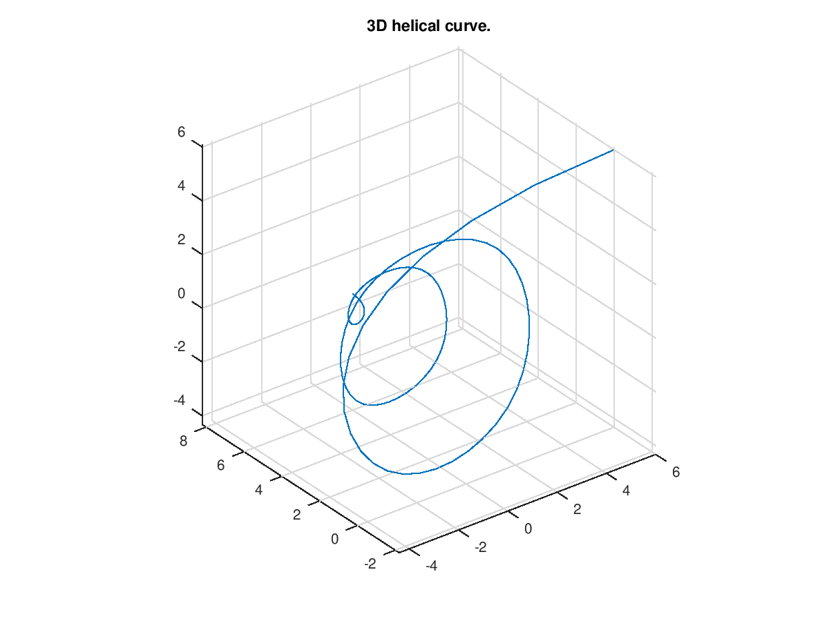
Demonstration 4
The following code
 coefs =[ 6.0  0.0  6.0  1;
         -5.5  0.5  5.5  1;
         -5.0  1.0 -5.0  1;
          4.5  1.5 -4.5  1;
          4.0  2.0  4.0  1;
         -3.5  2.5  3.5  1;
         -3.0  3.0 -3.0  1;
          2.5  3.5 -2.5  1;
          2.0  4.0  2.0  1;
         -1.5  4.5  1.5  1;
         -1.0  5.0 -1.0  1;
          0.5  5.5 -0.5  1;
          0.0  6.0  0.0  1]';
 knots = [0 0 0 0 .1 .2 .3 .4 .5 .6 .7 .8 .9 1 1 1 1];

 crv = nrbmak(coefs,knots);
 nrbplot(crv,100);
 grid on;
 title('3D helical curve.');
 hold off
Produces the following figure
| Figure 1 |
|---|
 |
Package: nurbs