 NRBPLOT: Plot a NURBS curve or surface, or the boundary of a NURBS volume.

 Calling Sequence:

   nrbplot (nrb, npnts)
   nrbplot (nrb, npnts, p, v)

 INPUT:

   nrb		: NURBS curve, surface or volume, see nrbmak.

   npnts	: Number of evaluation points, for a surface or volume, a row
       vector with the number of points along each direction.

   [p,v]       : property/value options

               Valid property/value pairs include:

               Property        Value/{Default}
               -----------------------------------
               light           {off} | on
               colormap        {'copper'}

 Example:

   Plot the test surface with 20 points along the U direction
   and 30 along the V direction

   nrbplot(nrbtestsrf, [20 30])

    Copyright (C) 2000 Mark Spink
    Copyright (C) 2010 Carlo de Falco, Rafael Vazquez
    Copyright (C) 2012 Rafael Vazquez

    This program is free software: you can redistribute it and/or modify
    it under the terms of the GNU General Public License as published by
    the Free Software Foundation, either version 3 of the License, or
    (at your option) any later version.
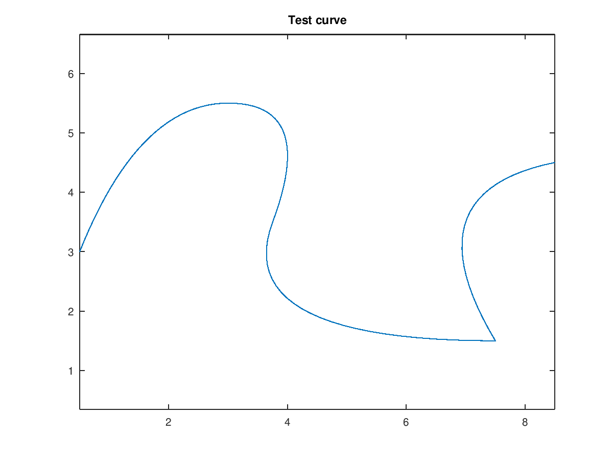
Demonstration 1
The following code
 crv = nrbtestcrv;
 nrbplot(crv,100)
 title('Test curve')
 hold off
Produces the following figure
| Figure 1 |
|---|
 |
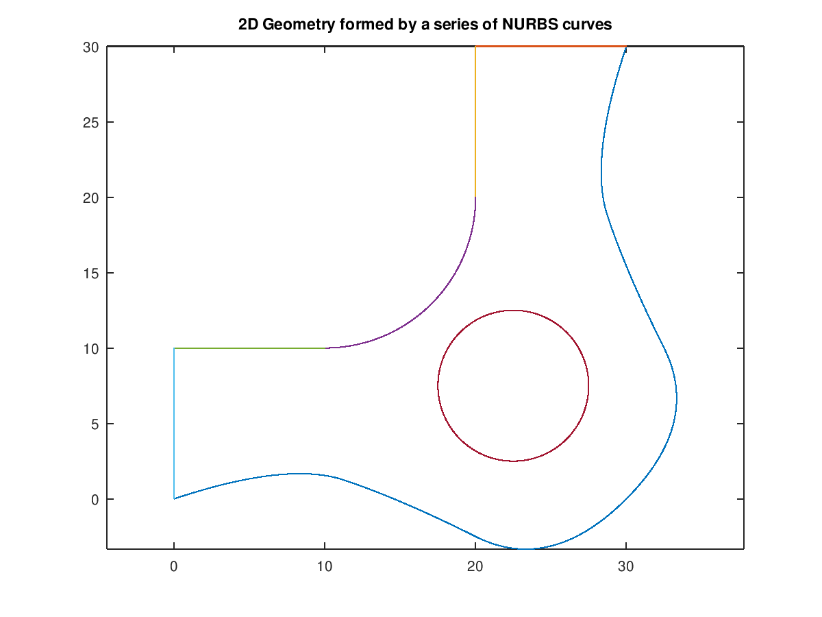
Demonstration 2
The following code
 coefs = [0.0 7.5 15.0 25.0 35.0 30.0 27.5 30.0;
          0.0 2.5  0.0 -5.0  5.0 15.0 22.5 30.0];
 knots = [0.0 0.0 0.0 1/6 1/3 1/2 2/3 5/6 1.0 1.0 1.0];

 geom = [
 nrbmak(coefs,knots)
 nrbline([30.0 30.0],[20.0 30.0])
 nrbline([20.0 30.0],[20.0 20.0])
 nrbcirc(10.0,[10.0 20.0],1.5*pi,0.0)
 nrbline([10.0 10.0],[0.0 10.0])
 nrbline([0.0 10.0],[0.0 0.0])
 nrbcirc(5.0,[22.5 7.5])
 ];

 ng = length(geom);
 for i = 1:ng
   nrbplot(geom(i),500);
   hold on;
 end
 hold off;
 axis equal;
 title('2D Geometry formed by a series of NURBS curves');
Produces the following figure
| Figure 1 |
|---|
 |
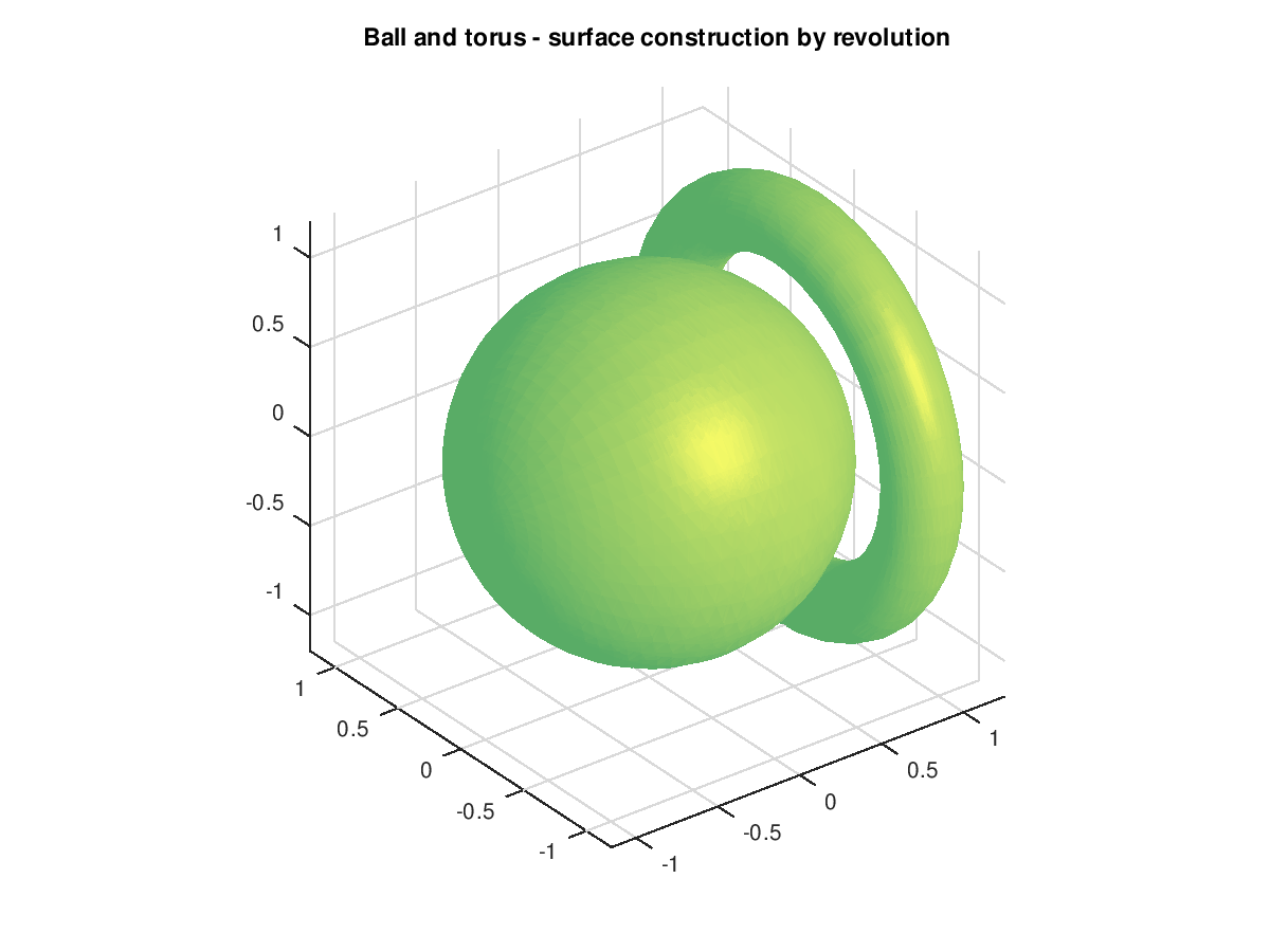
Demonstration 3
The following code
 sphere = nrbrevolve(nrbcirc(1,[],0.0,pi),[0.0 0.0 0.0],[1.0 0.0 0.0]);
 nrbplot(sphere,[40 40],'light','on');
 title('Ball and torus - surface construction by revolution');
 hold on;
 torus = nrbrevolve(nrbcirc(0.2,[0.9 1.0]),[0.0 0.0 0.0],[1.0 0.0 0.0]);
 nrbplot(torus,[40 40],'light','on');
 hold off
Produces the following figure
| Figure 1 |
|---|
 |
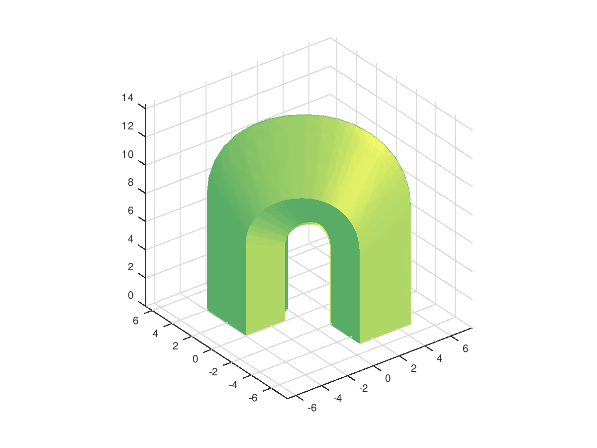
Demonstration 4
The following code
 knots = {[0 0 0 1/2 1 1 1] [0 0 0 1 1 1]...
          [0 0 0 1/6 2/6 1/2 1/2 4/6 5/6 1 1 1]};

 coefs = [-1.0000   -0.9734   -0.7071    1.4290    1.0000    3.4172
          0    2.4172         0    0.0148   -2.0000   -1.9734
          0    2.0000    4.9623    9.4508    4.0000    2.0000
     1.0000    1.0000    0.7071    1.0000    1.0000    1.0000
    -0.8536         0   -0.6036    1.9571    1.2071    3.5000
     0.3536    2.5000    0.2500    0.5429   -1.7071   -1.0000
          0    2.0000    4.4900    8.5444    3.4142    2.0000
     0.8536    1.0000    0.6036    1.0000    0.8536    1.0000
    -0.3536   -4.0000   -0.2500   -1.2929    1.7071    1.0000
     0.8536         0    0.6036   -2.7071   -1.2071   -5.0000
          0    2.0000    4.4900   10.0711    3.4142    2.0000
     0.8536    1.0000    0.6036    1.0000    0.8536    1.0000
          0   -4.0000         0    0.7071    2.0000    5.0000
     1.0000    4.0000    0.7071   -0.7071   -1.0000   -5.0000
          0    2.0000    4.9623   14.4142    4.0000    2.0000
     1.0000    1.0000    0.7071    1.0000    1.0000    1.0000
    -2.5000   -4.0000   -1.7678    0.7071    1.0000    5.0000
          0    4.0000         0   -0.7071   -3.5000   -5.0000
          0    2.0000    6.0418   14.4142    4.0000    2.0000
     1.0000    1.0000    0.7071    1.0000    1.0000    1.0000
    -2.4379         0   -1.7238    2.7071    1.9527    5.0000
     0.9527    4.0000    0.6737    1.2929   -3.4379   -1.0000
          0    2.0000    6.6827   10.0711    4.0000    2.0000
     1.0000    1.0000    0.7071    1.0000    1.0000    1.0000
    -0.9734   -1.0000   -0.6883    0.7071    3.4172    1.0000
     2.4172         0    1.7092   -1.4142   -1.9734   -2.0000
          0    4.0000    6.6827    4.9623    4.0000         0
     1.0000    1.0000    0.7071    0.7071    1.0000    1.0000
          0   -0.8536         0    0.8536    3.5000    1.2071
     2.5000    0.3536    1.7678   -1.2071   -1.0000   -1.7071
          0    3.4142    6.0418    4.4900    4.0000         0
     1.0000    0.8536    0.7071    0.6036    1.0000    0.8536
    -4.0000   -0.3536   -2.8284    1.2071    1.0000    1.7071
          0    0.8536         0   -0.8536   -5.0000   -1.2071
          0    3.4142    7.1213    4.4900    4.0000         0
     1.0000    0.8536    0.7071    0.6036    1.0000    0.8536
    -4.0000         0   -2.8284    1.4142    5.0000    2.0000
     4.0000    1.0000    2.8284   -0.7071   -5.0000   -1.0000
          0    4.0000   10.1924    4.9623    4.0000         0
     1.0000    1.0000    0.7071    0.7071    1.0000    1.0000
    -4.0000   -2.5000   -2.8284    0.7071    5.0000    1.0000
     4.0000         0    2.8284   -2.4749   -5.0000   -3.5000
          0    4.0000   10.1924    6.0418    4.0000         0
     1.0000    1.0000    0.7071    0.7071    1.0000    1.0000
          0   -2.4379         0    1.3808    5.0000    1.9527
     4.0000    0.9527    2.8284   -2.4309   -1.0000   -3.4379
          0    4.0000    7.1213    6.6827    4.0000         0
     1.0000    1.0000    0.7071    0.7071    1.0000    1.0000
    -1.0000   -0.9734    0.2071    2.4163    1.0000    3.4172
          0    2.4172   -1.2071   -1.3954   -2.0000   -1.9734
     2.0000    4.0000    7.0178    6.6827    2.0000         0
     1.0000    1.0000    1.0000    0.7071    1.0000    1.0000
    -0.8536         0    0.3536    2.4749    1.2071    3.5000
     0.3536    2.5000   -0.8536   -0.7071   -1.7071   -1.0000
     1.7071    4.0000    6.3498    6.0418    1.7071         0
     0.8536    1.0000    0.8536    0.7071    0.8536    1.0000
    -0.3536   -4.0000    0.8536    0.7071    1.7071    1.0000
     0.8536         0   -0.3536   -3.5355   -1.2071   -5.0000
     1.7071    4.0000    6.3498    7.1213    1.7071         0
     0.8536    1.0000    0.8536    0.7071    0.8536    1.0000
          0   -4.0000    1.2071    3.5355    2.0000    5.0000
     1.0000    4.0000   -0.2071   -3.5355   -1.0000   -5.0000
     2.0000    4.0000    7.0178   10.1924    2.0000         0
     1.0000    1.0000    1.0000    0.7071    1.0000    1.0000
    -2.5000   -4.0000   -0.5429    3.5355    1.0000    5.0000
          0    4.0000   -1.9571   -3.5355   -3.5000   -5.0000
     2.0000    4.0000    8.5444   10.1924    2.0000         0
     1.0000    1.0000    1.0000    0.7071    1.0000    1.0000
    -2.4379         0   -0.0355    3.5355    1.9527    5.0000
     0.9527    4.0000   -1.4497   -0.7071   -3.4379   -1.0000
     2.0000    4.0000    9.4508    7.1213    2.0000         0
     1.0000    1.0000    1.0000    0.7071    1.0000    1.0000];
 coefs = reshape (coefs, 4, 4, 3, 9);
 horseshoe = nrbmak (coefs, knots);
 nrbplot (horseshoe, [6, 6, 50], 'light', 'on');
Produces the following figure
| Figure 1 |
|---|
 |
Package: nurbs