
|
Octave-Forge - Extra packages for GNU Octave |
| Home · Packages · Developers · Documentation · FAQ · Bugs · Mailing Lists · Links · Code |
|
|
Octave-Forge - Extra packages for GNU Octave |
| Home · Packages · Developers · Documentation · FAQ · Bugs · Mailing Lists · Links · Code |
Create a 2-D plot with errorbars.
Many different combinations of arguments are possible. The simplest form is
errorbar (y, ey)
where the first argument is taken as the set of y coordinates, the
second argument ey are the errors around the y values, and the
x coordinates are taken to be the indices of the elements
(1:numel (y)).
The general form of the function is
errorbar (x, y, err1, …, fmt, …)
After the x and y arguments there can be 1, 2, or 4 parameters specifying the error values depending on the nature of the error values and the plot format fmt.
When the error is a scalar all points share the same error value. The errorbars are symmetric and are drawn from data-err to data+err. The fmt argument determines whether err is in the x-direction, y-direction (default), or both.
Each data point has a particular error value. The errorbars are symmetric and are drawn from data(n)-err(n) to data(n)+err(n).
The errors have a single low-side value and a single upper-side value. The errorbars are not symmetric and are drawn from data-lerr to data+uerr.
Each data point has a low-side error and an upper-side error. The errorbars are not symmetric and are drawn from data(n)-lerr(n) to data(n)+uerr(n).
Any number of data sets (x1,y1, x2,y2, …) may appear as long as they are separated by a format string fmt.
If y is a matrix, x and the error parameters must also be matrices having the same dimensions. The columns of y are plotted versus the corresponding columns of x and errorbars are taken from the corresponding columns of the error parameters.
If fmt is missing, the yerrorbars ("~") plot style is assumed.
If the fmt argument is supplied then it is interpreted, as in normal plots, to specify the line style, marker, and color. In addition, fmt may include an errorbar style which must precede the ordinary format codes. The following errorbar styles are supported:
Set yerrorbars plot style (default).
Set xerrorbars plot style.
Set xyerrorbars plot style.
Set yboxes plot style.
Set xboxes plot style.
Set xyboxes plot style.
If the first argument hax is an axes handle, then plot into this axis,
rather than the current axes returned by gca.
The optional return value h is a handle to the hggroup object representing the data plot and errorbars.
Note: For compatibility with MATLAB a line is drawn through all data
points. However, most scientific errorbar plots are a scatter plot of
points with errorbars. To accomplish this, add a marker style to the
fmt argument such as ".". Alternatively, remove the line
by modifying the returned graphic handle with
set (h, "linestyle", "none").
Examples:
errorbar (x, y, ex, ">.r")
produces an xerrorbar plot of y versus x with x
errorbars drawn from x-ex to x+ex. The marker
"." is used so no connecting line is drawn and the errorbars
appear in red.
errorbar (x, y1, ey, "~",
          x, y2, ly, uy)
produces yerrorbar plots with y1 and y2 versus x. Errorbars for y1 are drawn from y1-ey to y1+ey, errorbars for y2 from y2-ly to y2+uy.
errorbar (x, y, lx, ux,
          ly, uy, "~>")
produces an xyerrorbar plot of y versus x in which x errorbars are drawn from x-lx to x+ux and y errorbars from y-ly to y+uy.
See also: semilogxerr, semilogyerr, loglogerr, plot.
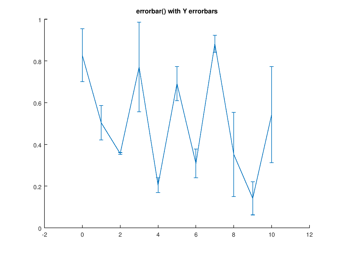
The following code
 clf;
 rand_1x11_data1 = [0.82712, 0.50325, 0.35613, 0.77089, 0.20474, 0.69160, 0.30858, 0.88225, 0.35187, 0.14168, 0.54270];
 rand_1x11_data2 = [0.506375, 0.330106, 0.017982, 0.859270, 0.140641, 0.327839, 0.275886, 0.162453, 0.807592, 0.318509, 0.921112];
 errorbar (0:10, rand_1x11_data1, 0.25*rand_1x11_data2);
 title ("errorbar() with Y errorbars");
Produces the following figure
| Figure 1 |
|---|
 |
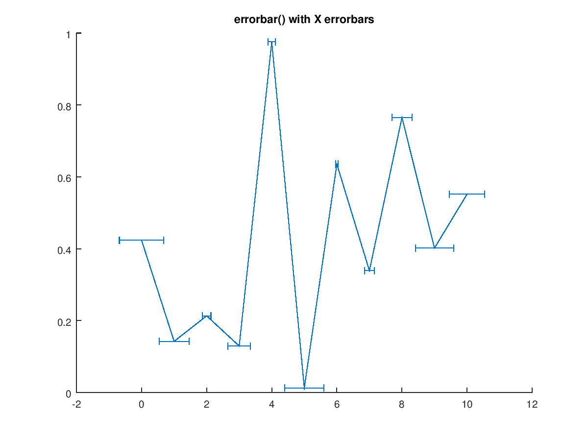
The following code
 clf;
 rand_1x11_data3 = [0.423650, 0.142331, 0.213195, 0.129301, 0.975891, 0.012872, 0.635327, 0.338829, 0.764997, 0.401798, 0.551850];
 rand_1x11_data4 = [0.682566, 0.456342, 0.132390, 0.341292, 0.108633, 0.601553, 0.040455, 0.146665, 0.309187, 0.586291, 0.540149];
 errorbar (0:10, rand_1x11_data3, rand_1x11_data4, ">");
 title ("errorbar() with X errorbars");
Produces the following figure
| Figure 1 |
|---|
 |
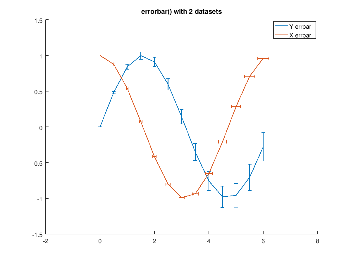
The following code
 clf;
 x = 0:0.5:2*pi;
 err = x/30;
 y1 = sin (x);
 y2 = cos (x);
 errorbar (x, y1, err, "~", x, y2, err, ">");
 legend ("Y errbar", "X errbar");
 title ("errorbar() with 2 datasets");
Produces the following figure
| Figure 1 |
|---|
 |
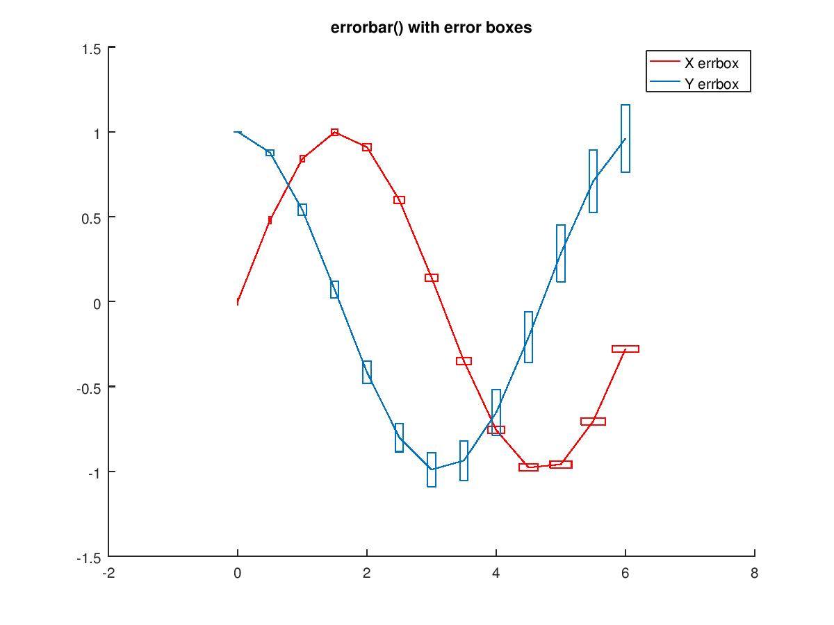
The following code
 clf;
 x = 0:0.5:2*pi;
 err = x/30;
 y1 = sin (x);
 y2 = cos (x);
 errorbar (x, y1, err, err, "#r", x, y2, err, err, "#~");
 legend ("X errbox", "Y errbox");
 title ("errorbar() with error boxes");
Produces the following figure
| Figure 1 |
|---|
 |
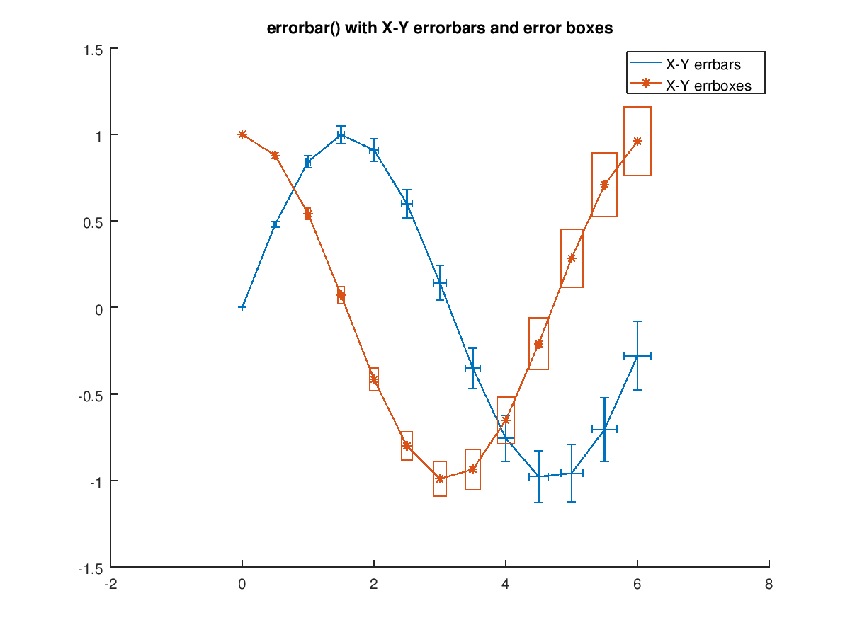
The following code
 clf;
 x = 0:0.5:2*pi;
 err = x/30;
 y1 = sin (x);
 y2 = cos (x);
 errorbar (x, y1, err, err, err, err, "~>", ...
           x, y2, err, err, err, err, "#~>-*");
 legend ("X-Y errbars", "X-Y errboxes");
 title ("errorbar() with X-Y errorbars and error boxes");
Produces the following figure
| Figure 1 |
|---|
 |
Package: octave