|
Octave-Forge - Extra packages for GNU Octave |
| Home · Packages · Developers · Documentation · FAQ · Bugs · Mailing Lists · Links · Code |
Plot a function fn within the range defined by limits.
fn is a function handle, inline function, or string containing the name of the function to evaluate.
The limits of the plot are of the form [xlo, xhi] or
[xlo, xhi, ylo, yhi].
The next three arguments are all optional and any number of them may be given in any order.
tol is the relative tolerance to use for the plot and defaults to 2e-3 (.2%).
n is the minimum number of points to use. When n is specified,
the maximum stepsize will be xhi - xlo / n. More
than n points may still be used in order to meet the relative
tolerance requirement.
The fmt argument specifies the linestyle to be used by the plot command.
If the first argument hax is an axes handle, then plot into this axis,
rather than the current axes returned by gca.
With no output arguments the results are immediately plotted. With two
output arguments the 2-D plot data is returned. The data can subsequently
be plotted manually with plot (x, y).
Example:
fplot (@cos, [0, 2*pi])
fplot ("[cos(x), sin(x)]", [0, 2*pi])
Programming Notes:
fplot works best with continuous functions. Functions with
discontinuities are unlikely to plot well. This restriction may be removed
in the future.
fplot requires that the function accept and return a vector argument.
Consider this when writing user-defined functions and use .*,
./, etc. See the function vectorize for potentially
converting inline or anonymous functions to vectorized versions.
See also: ezplot, plot, vectorize.
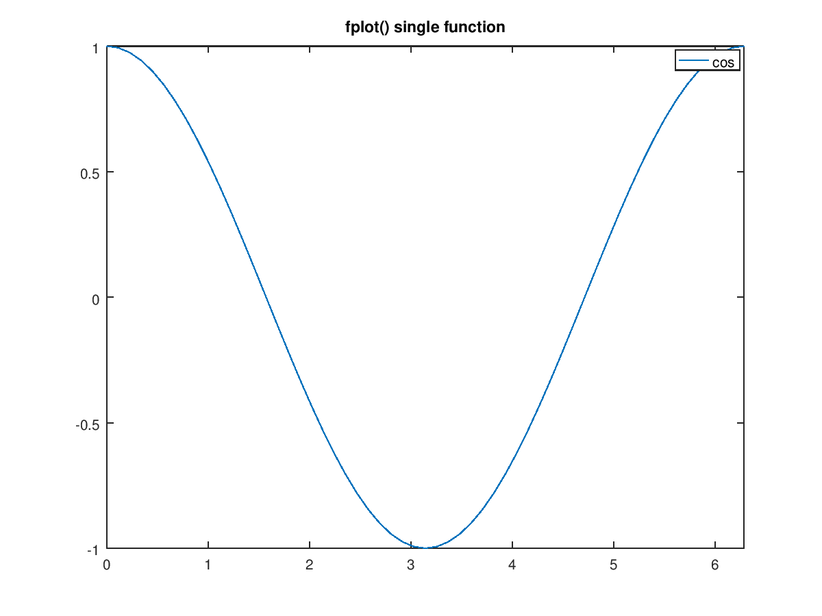
The following code
 clf;
 fplot (@cos, [0, 2*pi]);
 title ("fplot() single function");
Produces the following figure
| Figure 1 |
|---|
 |
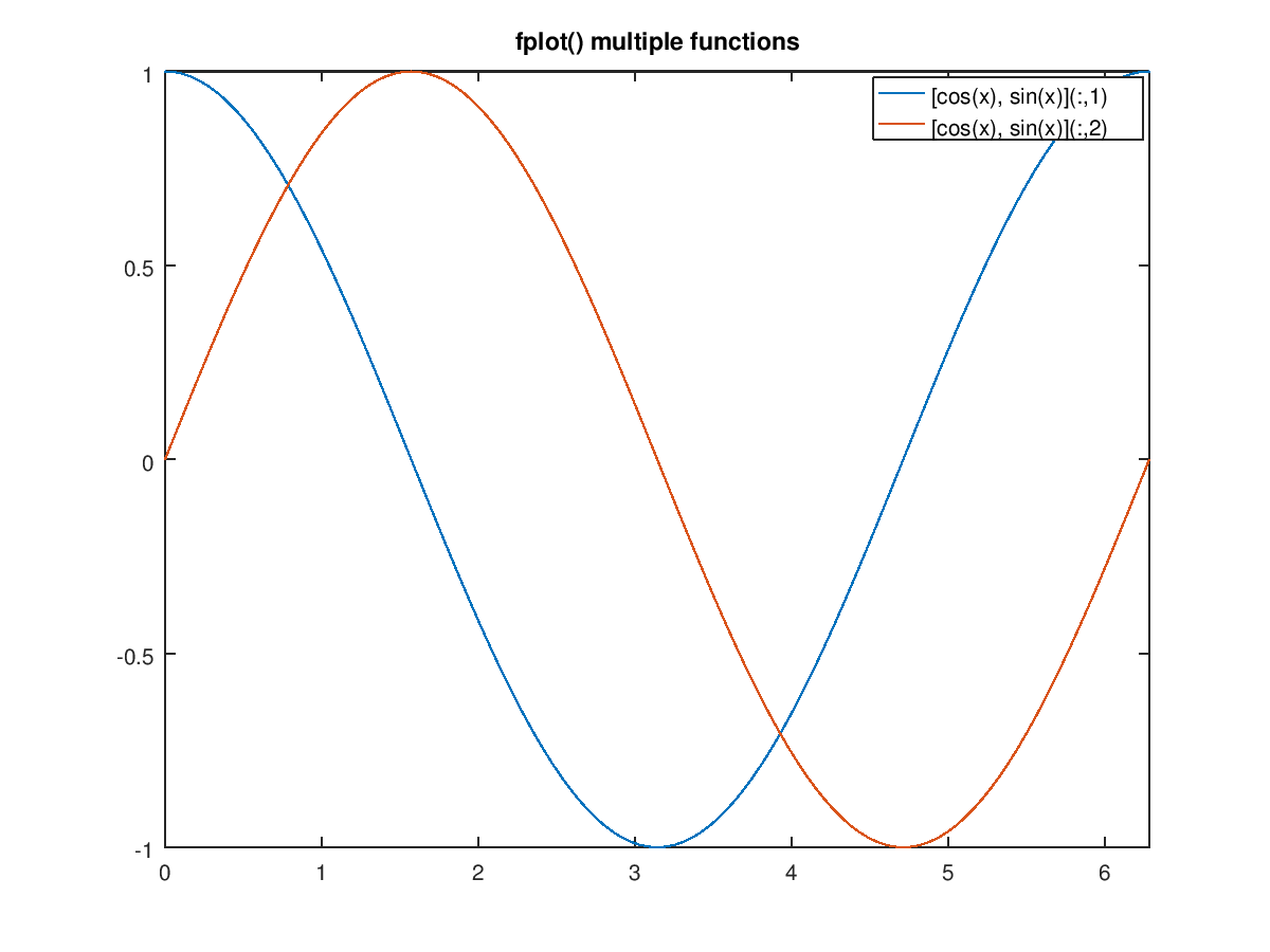
The following code
 clf;
 fplot ("[cos(x), sin(x)]", [0, 2*pi]);
 title ("fplot() multiple functions");
Produces the following figure
| Figure 1 |
|---|
 |
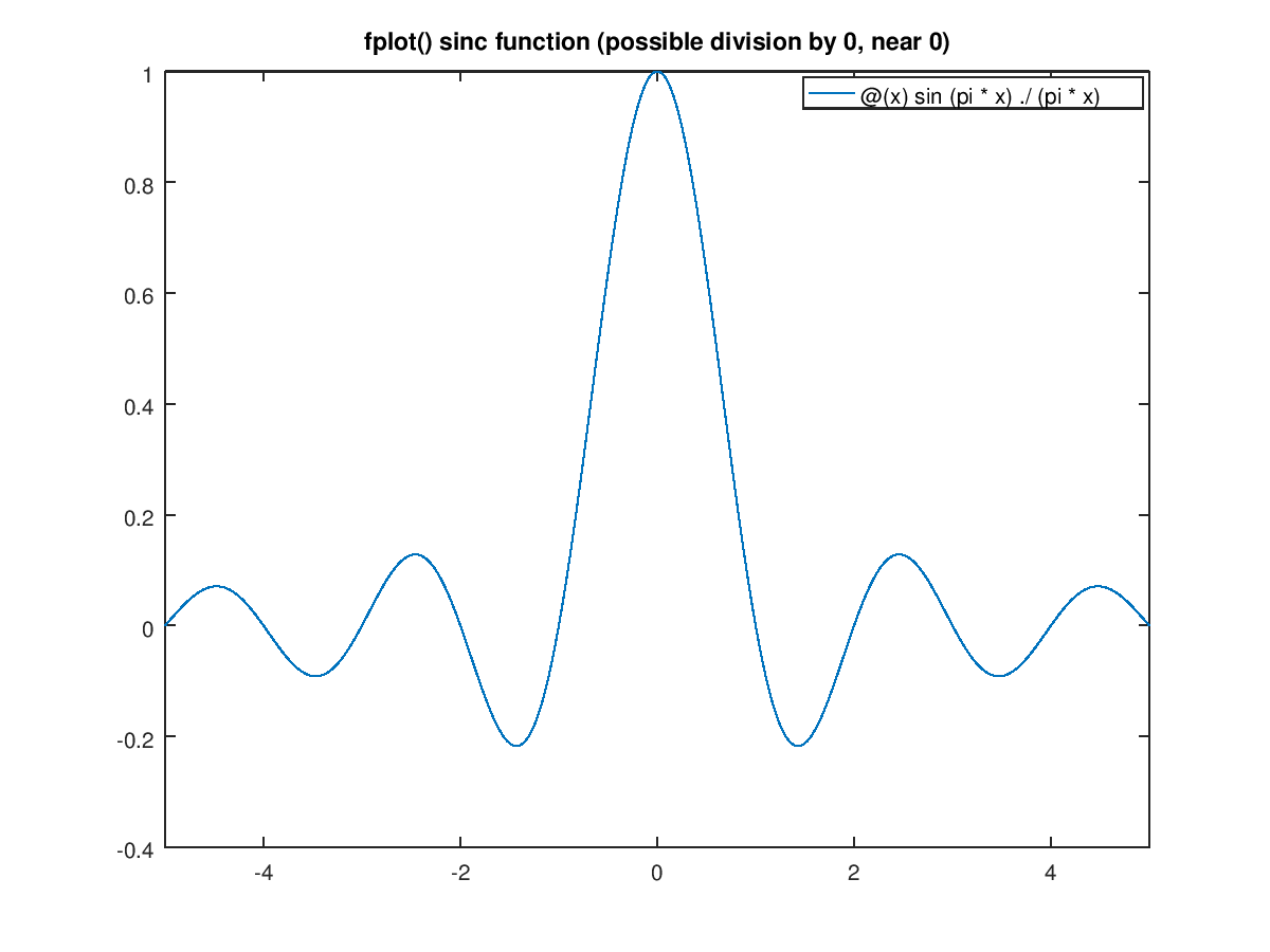
The following code
 clf;
 fh = @(x) sin (pi*x) ./ (pi*x);
 fplot (fh, [-5, 5]);
 title ("fplot() sinc function (possible division by 0, near 0)");
Produces the following figure
| Figure 1 |
|---|
 |
Package: octave