|
Octave-Forge - Extra packages for GNU Octave |
| Home · Packages · Developers · Documentation · FAQ · Bugs · Mailing Lists · Links · Code |
Display a matrix as an indexed color image.
The elements of img are indices into the current colormap.
x and y are optional 2-element vectors, [min, max],
which specify the range for the axis labels. If a range is specified as
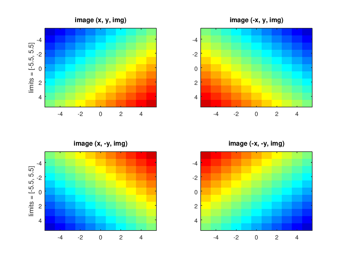
[max, min] then the image will be reversed along that axis. For
convenience, x and y may be specified as N-element vectors
matching the length of the data in img. However, only the first and
last elements will be used to determine the axis limits.
Multiple property/value pairs may be specified for the image object, but they must appear in pairs.
The optional return value h is a graphics handle to the image.
Implementation Note: The origin (0, 0) for images is located in the
upper left. For ordinary plots, the origin is located in the lower
left. Octave handles this inversion by plotting the data normally,
and then reversing the direction of the y-axis by setting the
ydir property to "reverse". This has implications whenever
an image and an ordinary plot need to be overlaid. The recommended
solution is to display the image and then plot the reversed ydata
using, for example, flipud (ydata).
Calling Forms: The image function can be called in two forms:
High-Level and Low-Level. When invoked with normal options, the High-Level
form is used which first calls newplot to prepare the graphic figure
and axes. When the only inputs to image are property/value pairs
the Low-Level form is used which creates a new instance of an image object
and inserts it in the current axes.
See also: imshow, imagesc, colormap.
The following code
 clf;
 colormap (jet (21));
 img = 1 ./ hilb (11);
 x = y = -5:5;
 subplot (2,2,1);
  h = image (x, y, img);
  ylabel ("limits = [-5.5, 5.5]");
  title ("image (x, y, img)");
 subplot (2,2,2);
  h = image (-x, y, img);
  title ("image (-x, y, img)");
 subplot (2,2,3);
  h = image (x, -y, img);
  title ("image (x, -y, img)");
  ylabel ("limits = [-5.5, 5.5]");
 subplot (2,2,4);
  h = image (-x, -y, img);
  title ("image (-x, -y, img)");
Produces the following figure
| Figure 1 |
|---|
 |
Package: octave