
|
Octave-Forge - Extra packages for GNU Octave |
| Home · Packages · Developers · Documentation · FAQ · Bugs · Mailing Lists · Links · Code |
|
|
Octave-Forge - Extra packages for GNU Octave |
| Home · Packages · Developers · Documentation · FAQ · Bugs · Mailing Lists · Links · Code |
One-dimensional interpolation.
Interpolate input data to determine the value of yi at the points
xi. If not specified, x is taken to be the indices of y
(1:length (y)). If y is a matrix or an N-dimensional
array, the interpolation is performed on each column of y.
The interpolation method is one of:
"nearest"Return the nearest neighbor.
"previous"Return the previous neighbor.
"next"Return the next neighbor.
"linear" (default)Linear interpolation from nearest neighbors.
"pchip"Piecewise cubic Hermite interpolating polynomial—shape-preserving interpolation with smooth first derivative.
"cubic"Cubic interpolation (same as "pchip").
"spline"Cubic spline interpolation—smooth first and second derivatives throughout the curve.
Adding ’*’ to the start of any method above forces interp1
to assume that x is uniformly spaced, and only x(1)
and x(2) are referenced. This is usually faster,
and is never slower. The default method is "linear".
If extrap is the string "extrap", then extrapolate values
beyond the endpoints using the current method. If extrap is a
number, then replace values beyond the endpoints with that number. When
unspecified, extrap defaults to NA.
If the string argument "pp" is specified, then xi should not
be supplied and interp1 returns a piecewise polynomial object. This
object can later be used with ppval to evaluate the interpolation.
There is an equivalence, such that ppval (interp1 (x,
y, method, .
"pp"), xi) == interp1 (x,
y, xi, method, "extrap")
Duplicate points in x specify a discontinuous interpolant. There
may be at most 2 consecutive points with the same value.
If x is increasing, the default discontinuous interpolant is
right-continuous. If x is decreasing, the default discontinuous
interpolant is left-continuous.
The continuity condition of the interpolant may be specified by using
the options "left" or "right" to select a left-continuous
or right-continuous interpolant, respectively.
Discontinuous interpolation is only allowed for "nearest" and
"linear" methods; in all other cases, the x-values must be
unique.
An example of the use of interp1 is
xf = [0:0.05:10];
yf = sin (2*pi*xf/5);
xp = [0:10];
yp = sin (2*pi*xp/5);
lin = interp1 (xp, yp, xf);
near = interp1 (xp, yp, xf, "nearest");
pch = interp1 (xp, yp, xf, "pchip");
spl = interp1 (xp, yp, xf, "spline");
plot (xf,yf,"r", xf,near,"g", xf,lin,"b", xf,pch,"c", xf,spl,"m",
      xp,yp,"r*");
legend ("original", "nearest", "linear", "pchip", "spline");
See also: pchip, spline, interpft, interp2, interp3, interpn.
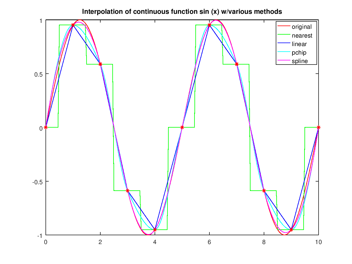
The following code
 clf;
 xf = 0:0.05:10;  yf = sin (2*pi*xf/5);
 xp = 0:10;       yp = sin (2*pi*xp/5);
 lin = interp1 (xp,yp,xf, 'linear');
 spl = interp1 (xp,yp,xf, 'spline');
 pch = interp1 (xp,yp,xf, 'pchip');
 near= interp1 (xp,yp,xf, 'nearest');
 plot (xf,yf,'r',xf,near,'g',xf,lin,'b',xf,pch,'c',xf,spl,'m',xp,yp,'r*');
 legend ('original', 'nearest', 'linear', 'pchip', 'spline');
 title ('Interpolation of continuous function sin (x) w/various methods');
 %--------------------------------------------------------
 % confirm that interpolated function matches the original
Produces the following figure
| Figure 1 |
|---|
 |
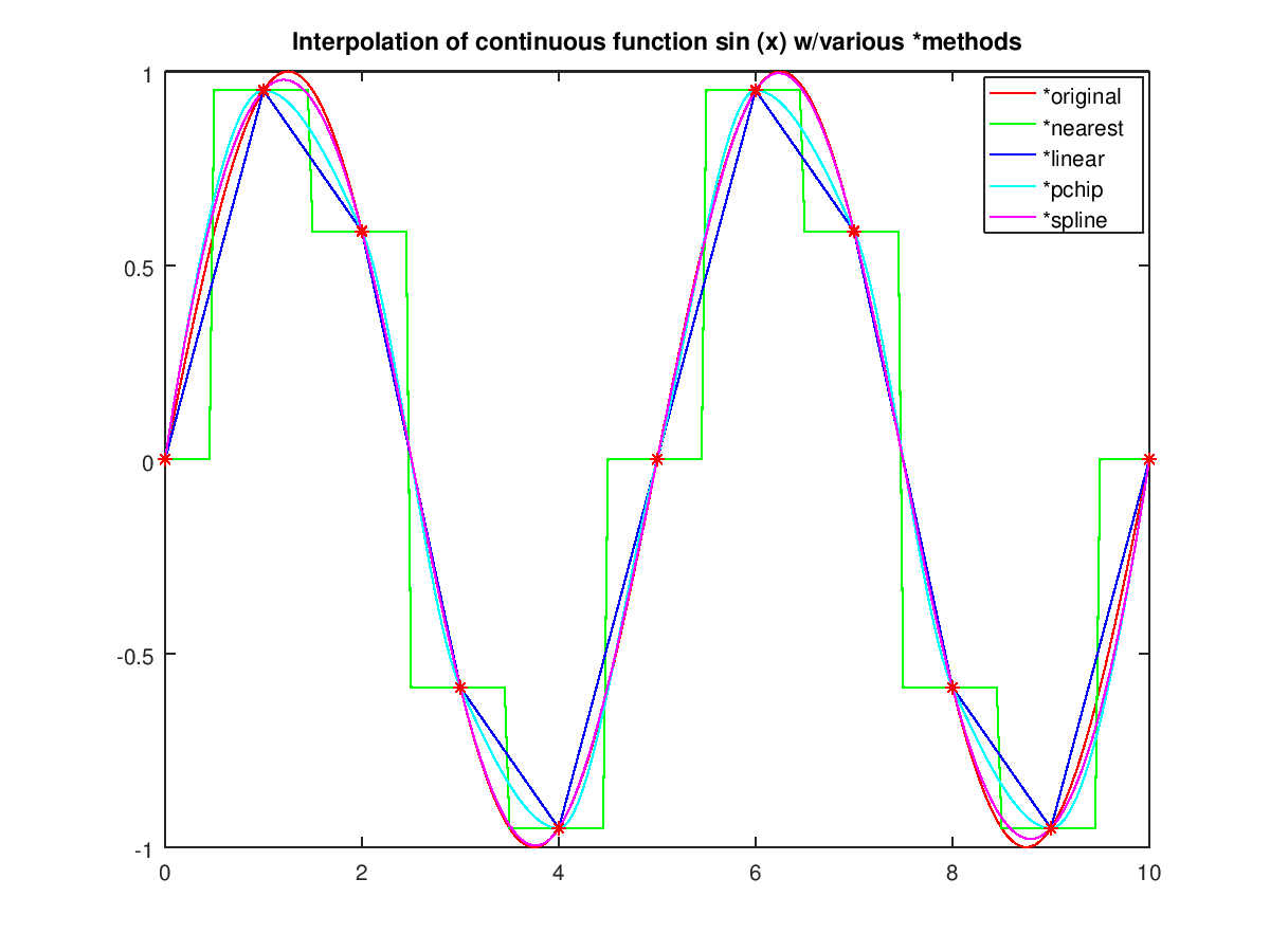
The following code
 clf;
 xf = 0:0.05:10;  yf = sin (2*pi*xf/5);
 xp = 0:10;       yp = sin (2*pi*xp/5);
 lin = interp1 (xp,yp,xf, '*linear');
 spl = interp1 (xp,yp,xf, '*spline');
 pch = interp1 (xp,yp,xf, '*pchip');
 near= interp1 (xp,yp,xf, '*nearest');
 plot (xf,yf,'r',xf,near,'g',xf,lin,'b',xf,pch,'c',xf,spl,'m',xp,yp,'r*');
 legend ('*original', '*nearest', '*linear', '*pchip', '*spline');
 title ('Interpolation of continuous function sin (x) w/various *methods');
 %--------------------------------------------------------
 % confirm that interpolated function matches the original
Produces the following figure
| Figure 1 |
|---|
 |
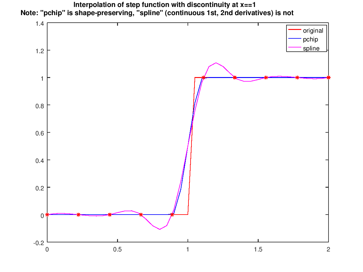
The following code
 clf;
 fstep = @(x) x > 1;
 xf = 0:0.05:2;  yf = fstep (xf);
 xp = linspace (0,2,10);  yp = fstep (xp);
 pch = interp1 (xp,yp,xf, 'pchip');
 spl = interp1 (xp,yp,xf, 'spline');
 plot (xf,yf,'r',xf,pch,'b',xf,spl,'m',xp,yp,'r*');
 title ({'Interpolation of step function with discontinuity at x==1', ...
         'Note: "pchip" is shape-preserving, "spline" (continuous 1st, 2nd derivatives) is not'});
 legend ('original', 'pchip', 'spline');
Produces the following figure
| Figure 1 |
|---|
 |
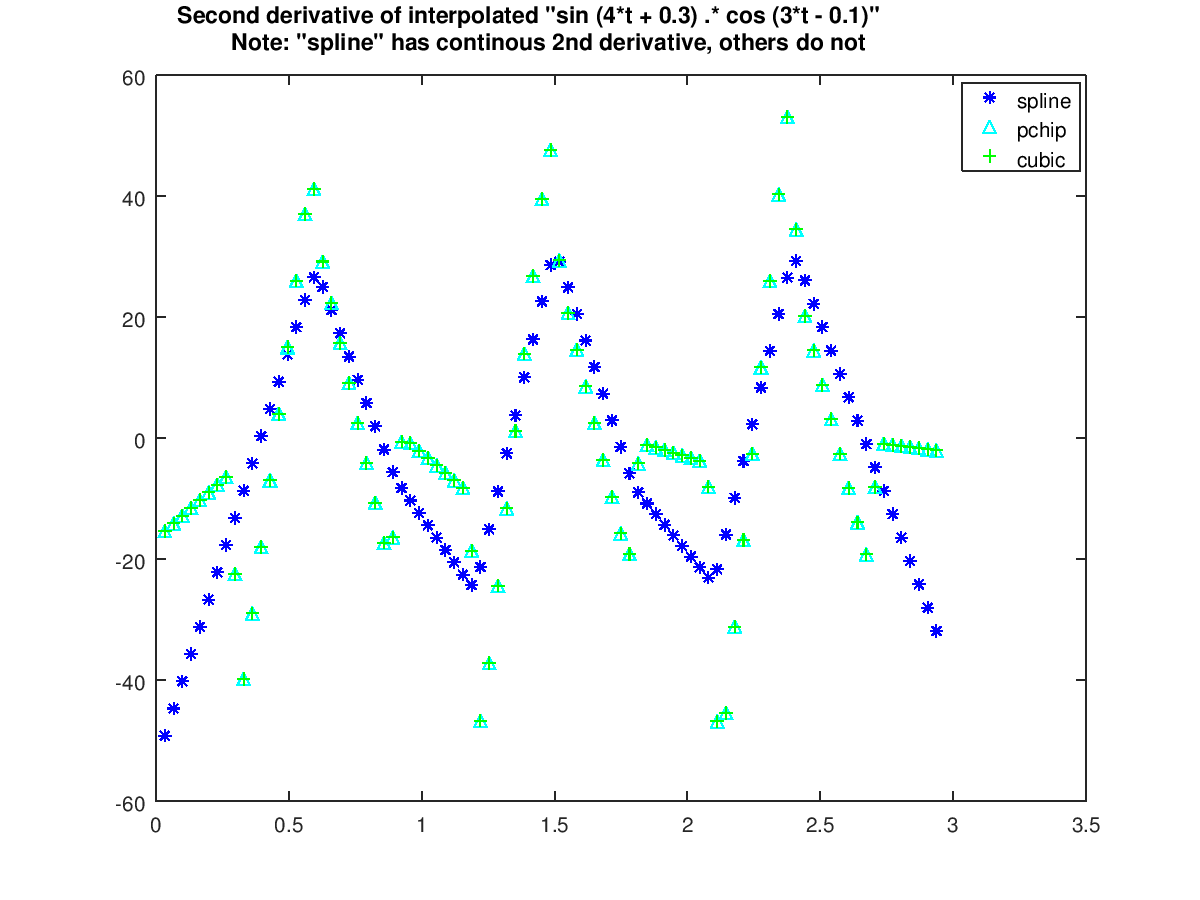
The following code
 clf;
 t = 0 : 0.3 : pi; dt = t(2)-t(1);
 n = length (t); k = 100; dti = dt*n/k;
 ti = t(1) + [0 : k-1]*dti;
 y = sin (4*t + 0.3) .* cos (3*t - 0.1);
 ddys = diff (diff (interp1 (t,y,ti, 'spline'))./dti)./dti;
 ddyp = diff (diff (interp1 (t,y,ti, 'pchip')) ./dti)./dti;
 ddyc = diff (diff (interp1 (t,y,ti, 'cubic')) ./dti)./dti;
 plot (ti(2:end-1),ddys,'b*', ti(2:end-1),ddyp,'c^', ti(2:end-1),ddyc,'g+');
 title ({'Second derivative of interpolated "sin (4*t + 0.3) .* cos (3*t - 0.1)"', ...
         'Note: "spline" has continous 2nd derivative, others do not'});
 legend ('spline', 'pchip', 'cubic');
Produces the following figure
| Figure 1 |
|---|
 |
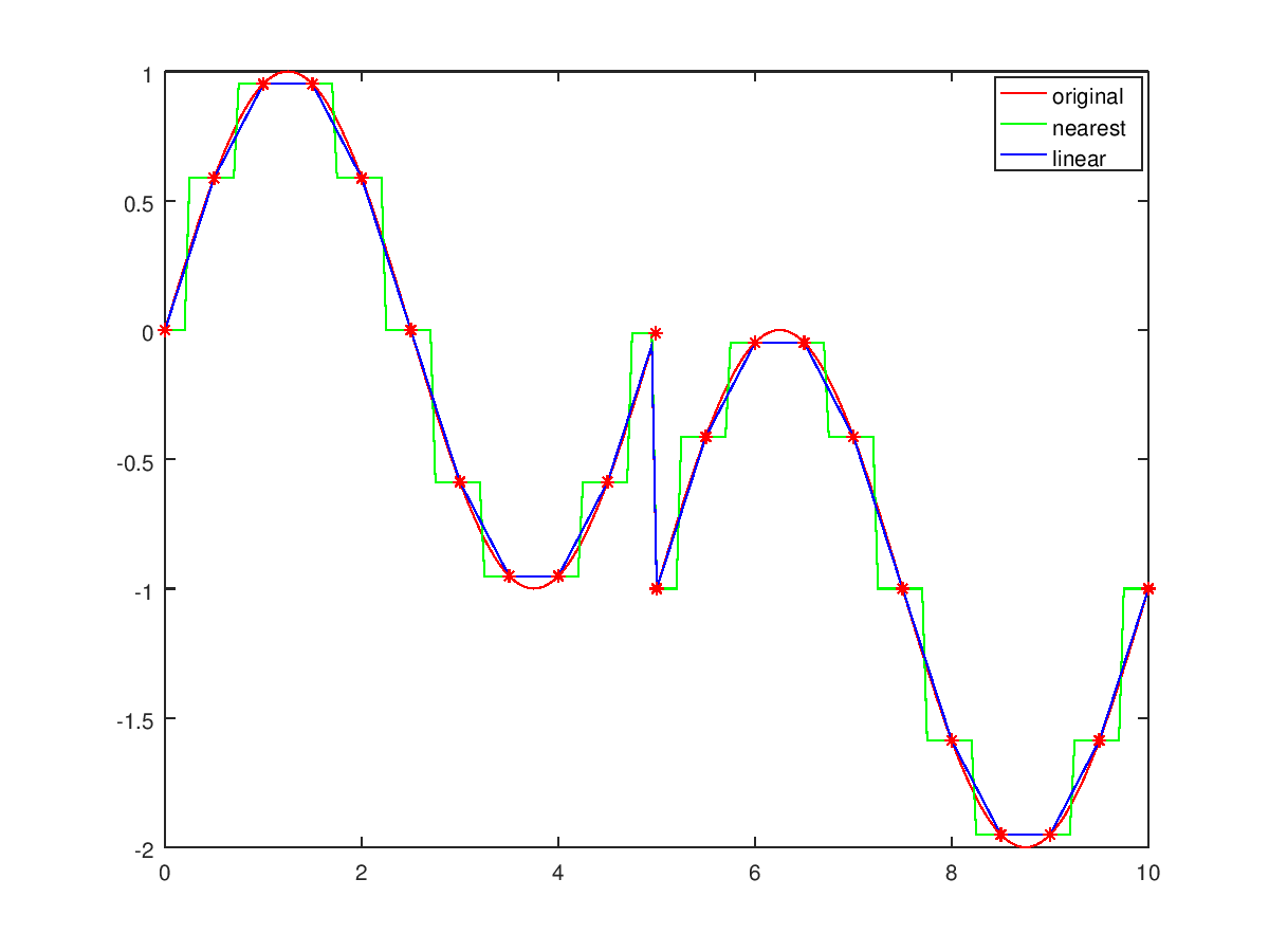
The following code
 clf;
 xf = 0:0.05:10;                yf = sin (2*pi*xf/5) - (xf >= 5);
 xp = [0:.5:4.5,4.99,5:.5:10];  yp = sin (2*pi*xp/5) - (xp >= 5);
 lin = interp1 (xp,yp,xf, 'linear');
 near= interp1 (xp,yp,xf, 'nearest');
 plot (xf,yf,'r', xf,near,'g', xf,lin,'b', xp,yp,'r*');
 legend ('original', 'nearest', 'linear');
 %--------------------------------------------------------
 % confirm that interpolated function matches the original
Produces the following figure
| Figure 1 |
|---|
 |
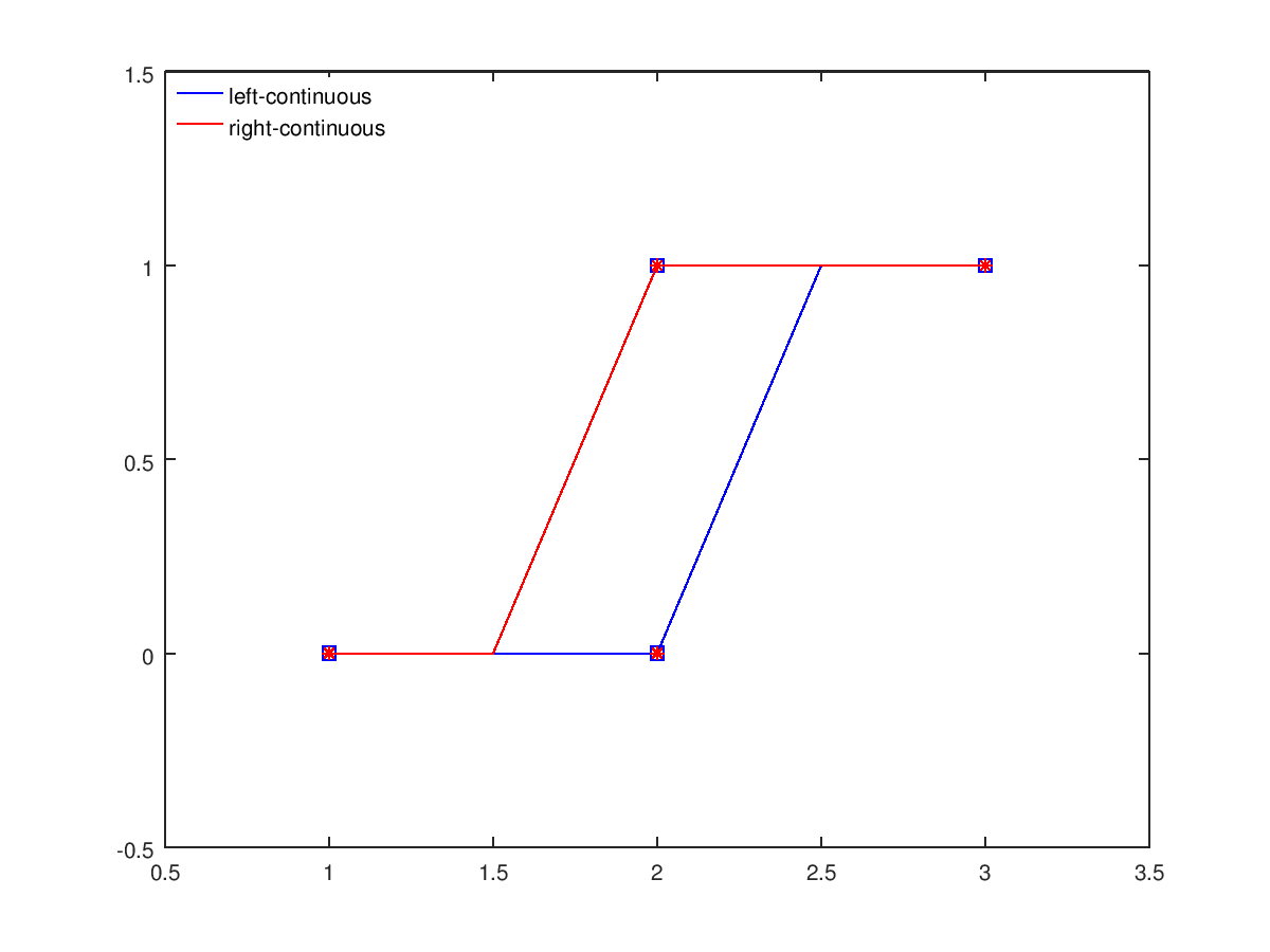
The following code
 clf;
 x = 0:0.5:3;
 x1 = [3 2 2 1];
 x2 = [1 2 2 3];
 y1 = [1 1 0 0];
 y2 = [0 0 1 1];
 h = plot (x, interp1 (x1, y1, x), 'b', x1, y1, 'sb');
 hold on
 g = plot (x, interp1 (x2, y2, x), 'r', x2, y2, '*r');
 axis ([0.5 3.5 -0.5 1.5]);
 legend ([h(1), g(1)], {'left-continuous', 'right-continuous'}, ...
         'location', 'northwest')
 legend boxoff
 %--------------------------------------------------------
 % red curve is left-continuous and blue is right-continuous at x = 2
Produces the following figure
| Figure 1 |
|---|
 |
Package: octave