
|
Octave-Forge - Extra packages for GNU Octave |
| Home · Packages · Developers · Documentation · FAQ · Bugs · Mailing Lists · Links · Code |
|
|
Octave-Forge - Extra packages for GNU Octave |
| Home · Packages · Developers · Documentation · FAQ · Bugs · Mailing Lists · Links · Code |
Perform n-dimensional interpolation, where n is at least two.
Each element of the n-dimensional array v represents a value
at a location given by the parameters x1, x2, …, xn.
The parameters x1, x2, …, xn are either
n-dimensional arrays of the same size as the array v in
the "ndgrid" format or vectors. The parameters y1, etc.
respect a similar format to x1, etc., and they represent the points
at which the array vi is interpolated.
If x1, …, xn are omitted, they are assumed to be
x1 = 1 : size (v, 1), etc. If m is specified, then
the interpolation adds a point half way between each of the interpolation
points. This process is performed m times. If only v is
specified, then m is assumed to be 1.
The interpolation method is one of:
"nearest"Return the nearest neighbor.
"linear" (default)Linear interpolation from nearest neighbors.
"pchip"Piecewise cubic Hermite interpolating polynomial—shape-preserving interpolation with smooth first derivative (not implemented yet).
"cubic"Cubic interpolation (same as "pchip" [not implemented yet]).
"spline"Cubic spline interpolation—smooth first and second derivatives throughout the curve.
The default method is "linear".
extrapval is a scalar number. It replaces values beyond the endpoints
with extrapval. Note that if extrapval is used, method
must be specified as well. If extrapval is omitted and the
method is "spline", then the extrapolated values of the
"spline" are used. Otherwise the default extrapval value for
any other method is "NA".
See also: interp1, interp2, interp3, spline, ndgrid.
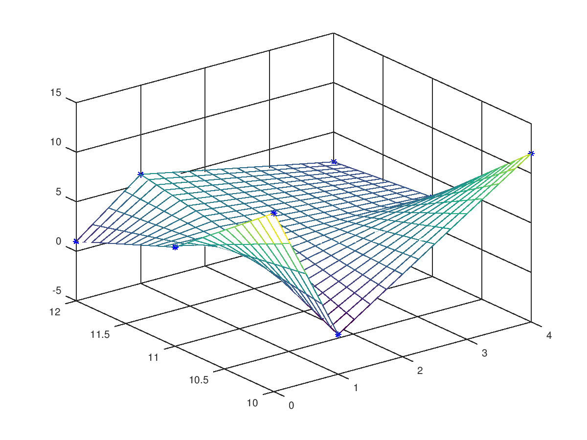
The following code
 clf;
 colormap ("default");
 A = [13,-1,12;5,4,3;1,6,2];
 x = [0,1,4];  y = [10,11,12];
 xi = linspace (min (x), max (x), 17);
 yi = linspace (min (y), max (y), 26)';
 mesh (xi, yi, interpn (x,y,A.',xi,yi, "linear").');
 [x,y] = meshgrid (x,y);
 hold on; plot3 (x(:),y(:),A(:),"b*"); hold off;
Produces the following figure
| Figure 1 |
|---|
 |
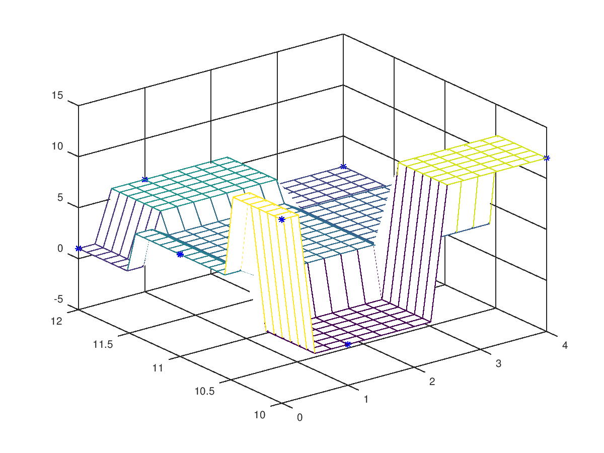
The following code
 clf;
 colormap ("default");
 A = [13,-1,12;5,4,3;1,6,2];
 x = [0,1,4];  y = [10,11,12];
 xi = linspace (min (x), max (x), 17);
 yi = linspace (min (y), max (y), 26)';
 mesh (xi, yi, interpn (x,y,A.',xi,yi, "nearest").');
 [x,y] = meshgrid (x,y);
 hold on; plot3 (x(:),y(:),A(:),"b*"); hold off;
Produces the following figure
| Figure 1 |
|---|
 |
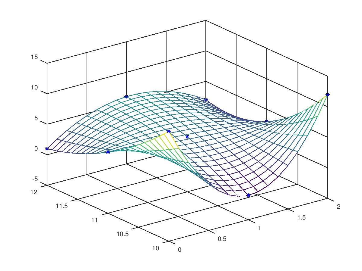
The following code
 clf;
 colormap ("default");
 A = [13,-1,12;5,4,3;1,6,2];
 x = [0,1,2];  y = [10,11,12];
 xi = linspace (min (x), max (x), 17);
 yi = linspace (min (y), max (y), 26)';
 mesh (xi, yi, interpn (x,y,A.',xi,yi, "spline").');
 [x,y] = meshgrid (x,y);
 hold on; plot3 (x(:),y(:),A(:),"b*"); hold off;
Produces the following figure
| Figure 1 |
|---|
 |
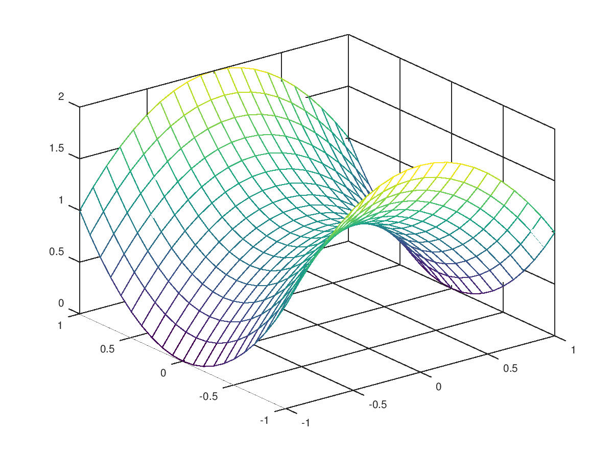
The following code
 clf;
 colormap ("default");
 x = y = z = -1:1;
 f = @(x,y,z) x.^2 - y - z.^2;
 [xx, yy, zz] = meshgrid (x, y, z);
 v = f (xx,yy,zz);
 xi = yi = zi = -1:0.1:1;
 [xxi, yyi, zzi] = ndgrid (xi, yi, zi);
 vi = interpn (x, y, z, v, xxi, yyi, zzi, "spline");
 mesh (yi, zi, squeeze (vi(1,:,:)));
Produces the following figure
| Figure 1 |
|---|
 |
Package: octave