
|
Octave-Forge - Extra packages for GNU Octave |
| Home · Packages · Developers · Documentation · FAQ · Bugs · Mailing Lists · Links · Code |
|
|
Octave-Forge - Extra packages for GNU Octave |
| Home · Packages · Developers · Documentation · FAQ · Bugs · Mailing Lists · Links · Code |
Calculate isosurface of 3-D volume data.
An isosurface connects points with the same value and is analogous to a contour plot, but in three dimensions.
The input argument v is a three-dimensional array that contains data sampled over a volume.
The input isoval is a scalar that specifies the value for the isosurface. If isoval is omitted or empty, a "good" value for an isosurface is determined from v.
When called with a single output argument isosurface returns a
structure array fv that contains the fields faces and
vertices computed at the points
[x, y, z] = meshgrid (1:l, 1:m, 1:n) where
[l, m, n] = size (v). The output fv can be
used directly as input to the patch function.
If called with additional input arguments x, y, and z
that are three-dimensional arrays with the same size as v or
vectors with lengths corresponding to the dimensions of v, then the
volume data is taken at the specified points. If x, y, or
z are empty, the grid corresponds to the indices (1:n) in
the respective direction (see ‘meshgrid’).
The optional input argument col, which is a three-dimensional array of the same size as v, specifies coloring of the isosurface. The color data is interpolated, as necessary, to match isoval. The output structure array, in this case, has the additional field facevertexcdata.
If given the string input argument "noshare", vertices may be
returned multiple times for different faces. The default behavior is to
eliminate vertices shared by adjacent faces with unique which may be
time consuming.
The string input argument "verbose" is supported for MATLAB
compatibility, but has no effect.
Any string arguments must be passed after the other arguments.
If called with two or three output arguments, return the information about the faces f, vertices v, and color data c as separate arrays instead of a single structure array.
If called with no output argument, the isosurface geometry is directly
plotted with the patch command and a light object is added to
the axes if not yet present.
For example,
[x, y, z] = meshgrid (1:5, 1:5, 1:5);
v = rand (5, 5, 5);
isosurface (x, y, z, v, .5);
will directly draw a random isosurface geometry in a graphics window.
An example of an isosurface geometry with different additional coloring:
N = 15;    # Increase number of vertices in each direction
iso = .4;  # Change isovalue to .1 to display a sphere
lin = linspace (0, 2, N);
[x, y, z] = meshgrid (lin, lin, lin);
v = abs ((x-.5).^2 + (y-.5).^2 + (z-.5).^2);
figure ();

subplot (2,2,1); view (-38, 20);
[f, vert] = isosurface (x, y, z, v, iso);
p = patch ("Faces", f, "Vertices", vert, "EdgeColor", "none");
pbaspect ([1 1 1]);
isonormals (x, y, z, v, p)
set (p, "FaceColor", "green", "FaceLighting", "gouraud");
light ("Position", [1 1 5]);

subplot (2,2,2); view (-38, 20);
p = patch ("Faces", f, "Vertices", vert, "EdgeColor", "blue");
pbaspect ([1 1 1]);
isonormals (x, y, z, v, p)
set (p, "FaceColor", "none", "EdgeLighting", "gouraud");
light ("Position", [1 1 5]);

subplot (2,2,3); view (-38, 20);
[f, vert, c] = isosurface (x, y, z, v, iso, y);
p = patch ("Faces", f, "Vertices", vert, "FaceVertexCData", c, ...
           "FaceColor", "interp", "EdgeColor", "none");
pbaspect ([1 1 1]);
isonormals (x, y, z, v, p)
set (p, "FaceLighting", "gouraud");
light ("Position", [1 1 5]);

subplot (2,2,4); view (-38, 20);
p = patch ("Faces", f, "Vertices", vert, "FaceVertexCData", c, ...
           "FaceColor", "interp", "EdgeColor", "blue");
pbaspect ([1 1 1]);
isonormals (x, y, z, v, p)
set (p, "FaceLighting", "gouraud");
light ("Position", [1 1 5]);
See also: isonormals, isocolors, isocaps, smooth3, reducevolume, reducepatch, patch.
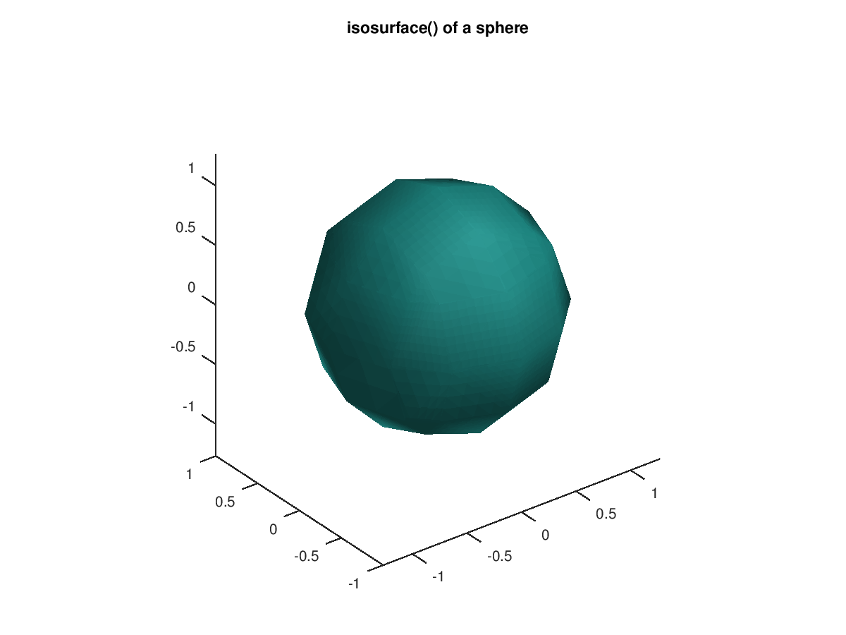
The following code
 clf;
 [x,y,z] = meshgrid (-2:0.5:2, -2:0.5:2, -2:0.5:2);
 v = x.^2 + y.^2 + z.^2;
 isosurface (x, y, z, v, 1);
 axis equal;
 title ("isosurface() of a sphere");
Produces the following figure
| Figure 1 |
|---|
 |
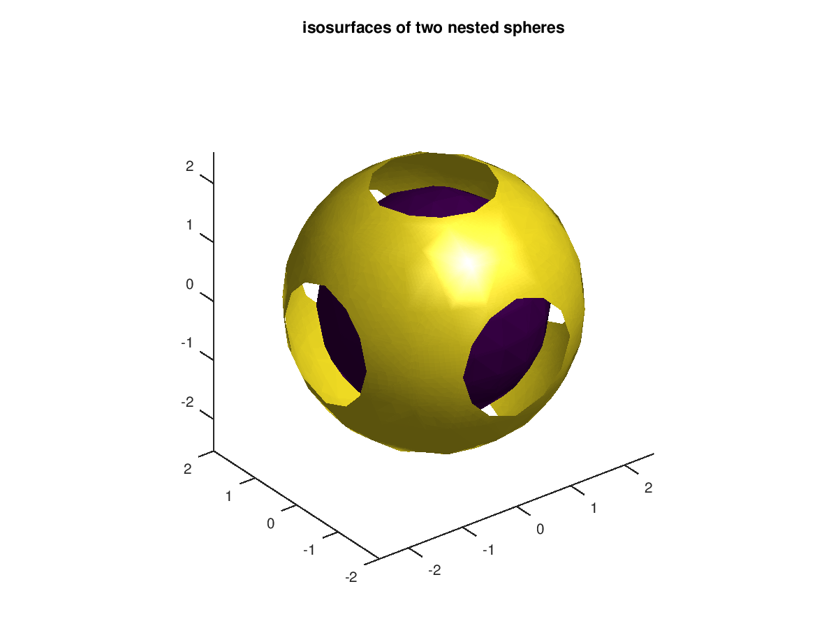
The following code
 clf;
 [x,y,z] = meshgrid (-2:0.5:2, -2:0.5:2, -2:0.5:2);
 v = x.^2 + y.^2 + z.^2;
 isosurface (x, y, z, v, 3);
 isosurface (x, y, z, v, 5);
 axis equal;
 title ("isosurfaces of two nested spheres");
Produces the following figure
| Figure 1 |
|---|
 |
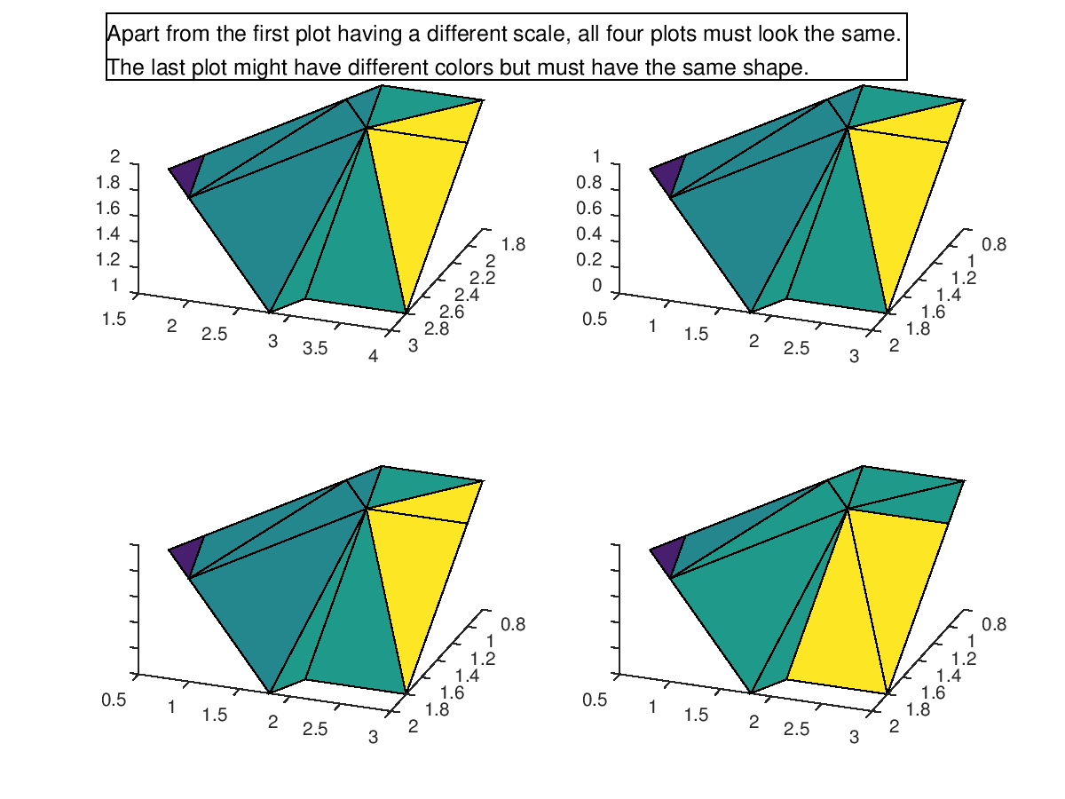
The following code
 x = 0:2;
 y = 0:3;
 z = 0:1;
 [xx, yy, zz] = meshgrid (x, y, z);
 v        = [0, 0, 0; 0, 0, 0; 0, 0, 1; 0, 0, 1];
 v(:,:,2) = [0, 0, 0; 0, 0, 1; 0, 1, 2; 0, 1, 2];
 iso = 0.8;
 clf;

 ## Three arguments, no output
 subplot (2, 2, 1);
  fvc = isosurface (v, iso, yy);
  patch (fvc);
  shading faceted;
  view (110, 40);
 ## six arguments, no output (x, y, z are vectors)
 subplot (2, 2, 2);
  fvc = isosurface (x, y, z, v, iso, yy);
  patch (fvc);
  shading faceted;
  view (110, 40);
 ## six arguments, no output (x, y, z are matrices)
 subplot (2, 2, 3);
  fvc = isosurface (xx, yy, zz, v, iso, yy);
  patch (fvc);
  shading faceted;
  view (110, 40);
 ## six arguments, no output (mixed x, y, z) and option "noshare"
 subplot (2, 2, 4);
  fvc = isosurface (x, yy, z, v, iso, yy, "noshare");
  patch (fvc);
  shading faceted;
  view (110, 40);
  annotation ("textbox", [0.1 0.9 0.9 0.1], ...
      "String", {["Apart from the first plot having a different scale, " ...
                  "all four plots must look the same."],
                 ["The last plot might have different colors but must " ...
                  "have the same shape."]}, ...
      "HorizontalAlignment", "left", ...
      "FontSize", 12);
Produces the following figure
| Figure 1 |
|---|
 |
Package: octave