
|
Octave-Forge - Extra packages for GNU Octave |
| Home · Packages · Developers · Documentation · FAQ · Bugs · Mailing Lists · Links · Code |
|
|
Octave-Forge - Extra packages for GNU Octave |
| Home · Packages · Developers · Documentation · FAQ · Bugs · Mailing Lists · Links · Code |
Solve a set of non-stiff Ordinary Differential Equations (non-stiff ODEs) with the well known explicit Bogacki-Shampine method of order 3. For the definition of this method see http://en.wikipedia.org/wiki/List_of_Runge%E2%80%93Kutta_methods.
fun is a function handle, inline function, or string containing the
name of the function that defines the ODE: y' = f(t,y). The function
must accept two inputs where the first is time t and the second is a
column vector of unknowns y.
trange specifies the time interval over which the ODE will be
evaluated. Typically, it is a two-element vector specifying the initial and
final times ([tinit, tfinal]). If there are more than two elements
then the solution will also be evaluated at these intermediate time
instances.
By default, ode23 uses an adaptive timestep with the
integrate_adaptive algorithm. The tolerance for the timestep
computation may be changed by using the options "RelTol"
and "AbsTol".
init contains the initial value for the unknowns. If it is a row vector then the solution y will be a matrix in which each column is the solution for the corresponding initial value in init.
The optional fourth argument ode_opt specifies non-default options to
the ODE solver. It is a structure generated by odeset.
The function typically returns two outputs. Variable t is a column vector and contains the times where the solution was found. The output y is a matrix in which each column refers to a different unknown of the problem and each row corresponds to a time in t.
The output can also be returned as a structure solution which
has a field x containing a row vector of times where the solution
was evaluated and a field y containing the solution matrix such
that each column corresponds to a time in x.
Use fieldnames (solution) to see the other fields and
additional information returned.
If using the "Events" option then three additional outputs may
be returned. te holds the time when an Event function returned a
zero. ye holds the value of the solution at time te. ie
contains an index indicating which Event function was triggered in the case
of multiple Event functions.
This function can be called with two output arguments: t and y. Variable t is a column vector and contains the time stamps, instead y is a matrix in which each column refers to a different unknown of the problem and the rows number is the same of t rows number so that each row of y contains the values of all unknowns at the time value contained in the corresponding row in t.
Example: Solve the Van der Pol equation
fvdp = @(t,y) [y(2); (1 - y(1)^2) * y(2) - y(1)];
[t,y] = ode23 (fvdp, [0, 20], [2, 0]);
See also: odeset, odeget, ode45.
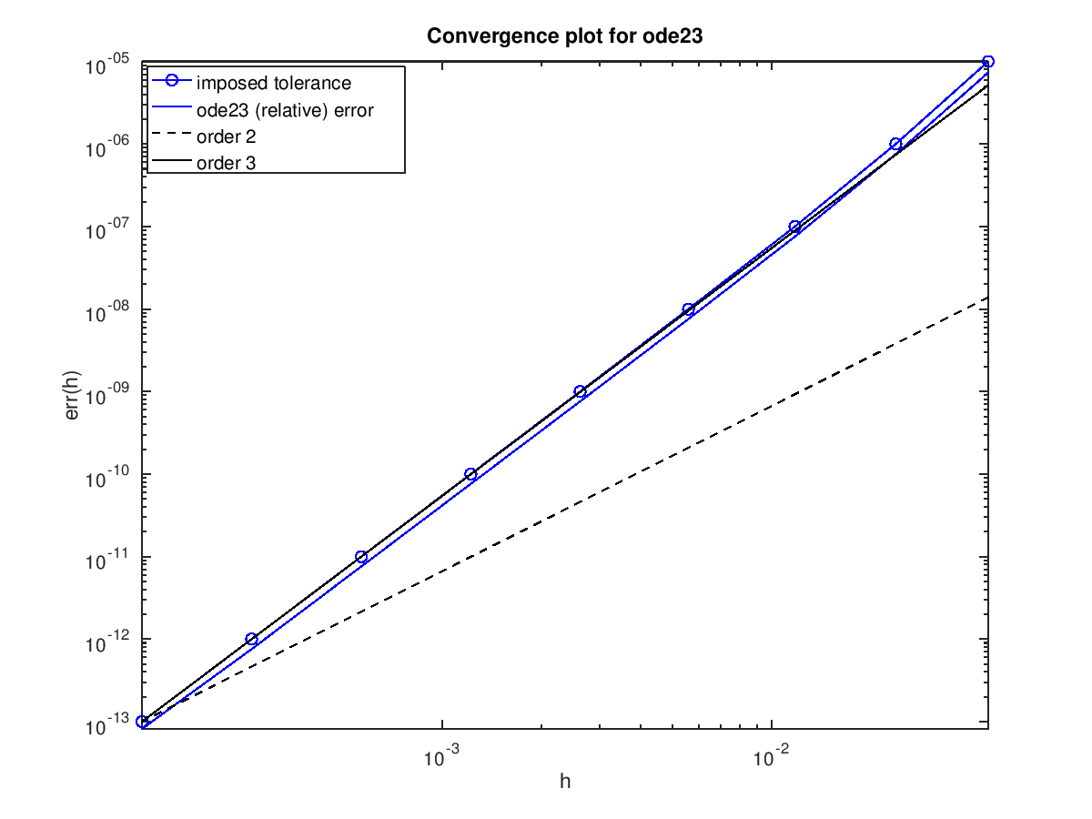
The following code
 ## Demonstrate convergence order for ode23
 tol = 1e-5 ./ 10.^[0:8];
 for i = 1 : numel (tol)
   opt = odeset ("RelTol", tol(i), "AbsTol", realmin);
   [t, y] = ode23 (@(t, y) -y, [0, 1], 1, opt);
   h(i) = 1 / (numel (t) - 1);
   err(i) = norm (y .* exp (t) - 1, Inf);
 endfor

 ## Estimate order visually
 loglog (h, tol, "-ob",
         h, err, "-b",
         h, (h/h(end)) .^ 2 .* tol(end), "k--",
         h, (h/h(end)) .^ 3 .* tol(end), "k-");
 axis tight
 xlabel ("h");
 ylabel ("err(h)");
 title ("Convergence plot for ode23");
 legend ("imposed tolerance", "ode23 (relative) error",
         "order 2", "order 3", "location", "northwest");

 ## Estimate order numerically
 p = diff (log (err)) ./ diff (log (h))
Produces the following output
p =

   3.5172   3.2636   3.0860   3.0353   3.0089   3.0088   3.0060   2.9026
and the following figure
| Figure 1 |
|---|
 |
Package: octave