
|
Octave-Forge - Extra packages for GNU Octave |
| Home · Packages · Developers · Documentation · FAQ · Bugs · Mailing Lists · Links · Code |
|
|
Octave-Forge - Extra packages for GNU Octave |
| Home · Packages · Developers · Documentation · FAQ · Bugs · Mailing Lists · Links · Code |
Open a new figure window and plot the solution of an ode problem at each time step during the integration.
The types and values of the input parameters t and y depend on the input flag that is of type string. Valid values of flag are:
"init"The input t must be a column vector of length 2 with the first and
last time step ([tfirst tlast]. The input y
contains the initial conditions for the ode problem (y0).
""The input t must be a scalar double specifying the time for which the solution in input y was calculated.
"done"The inputs should be empty, but are ignored if they are present.
odeplot always returns false, i.e., don’t stop the ode solver.
Example: solve an anonymous implementation of the
"Van der Pol" equation and display the results while
solving.
fvdp = @(t,y) [y(2); (1 - y(1)^2) * y(2) - y(1)];

opt = odeset ("OutputFcn", @odeplot, "RelTol", 1e-6);
sol = ode45 (fvdp, [0 20], [2 0], opt);
Background Information:
This function is called by an ode solver function if it was specified in
the "OutputFcn" property of an options structure created with
odeset. The ode solver will initially call the function with the
syntax odeplot ([tfirst, tlast], y0, "init"). The
function initializes internal variables, creates a new figure window, and
sets the x limits of the plot. Subsequently, at each time step during the
integration the ode solver calls odeplot (t, y, []).
At the end of the solution the ode solver calls
odeplot ([], [], "done") so that odeplot can perform any clean-up
actions required.
See also: odeset, odeget, ode23, ode45.
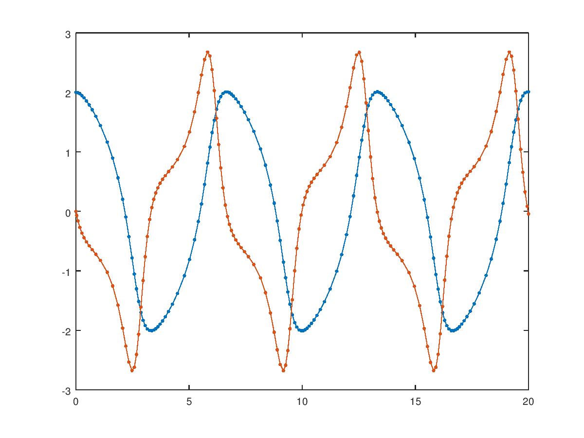
The following code
 ## Solve an anonymous implementation of the Van der Pol equation
 ## and display the results while solving
 fvdp = @(t,y) [y(2); (1 - y(1)^2) * y(2) - y(1)];
 opt = odeset ("OutputFcn", @odeplot, "RelTol", 1e-6);
 sol = ode45 (fvdp, [0 20], [2 0], opt);
Produces the following figure
| Figure 1 |
|---|
 |
Package: octave