
|
Octave-Forge - Extra packages for GNU Octave |
| Home · Packages · Developers · Documentation · FAQ · Bugs · Mailing Lists · Links · Code |
|
|
Octave-Forge - Extra packages for GNU Octave |
| Home · Packages · Developers · Documentation · FAQ · Bugs · Mailing Lists · Links · Code |
Produce 2-D plots.
Many different combinations of arguments are possible. The simplest form is
plot (y)
where the argument is taken as the set of y coordinates and the
x coordinates are taken to be the range 1:numel (y).
If more than one argument is given, they are interpreted as
plot (y, property, value, …)
or
plot (x, y, property, value, …)
or
plot (x, y, fmt, …)
and so on. Any number of argument sets may appear. The x and y values are interpreted as follows:
squeeze() is applied to arguments with more than two dimensions,
but no more than two singleton dimensions.
Multiple property-value pairs may be specified, but they must appear
in pairs. These arguments are applied to the line objects drawn by
plot. Useful properties to modify are "linestyle",
"linewidth", "color", "marker",
"markersize", "markeredgecolor", "markerfacecolor".
See ‘Line Properties’.
The fmt format argument can also be used to control the plot style.
It is a string composed of four optional parts:
"<linestyle><marker><color><;displayname;>".
When a marker is specified, but no linestyle, only the markers are
plotted. Similarly, if a linestyle is specified, but no marker, then
only lines are drawn. If both are specified then lines and markers will
be plotted. If no fmt and no property/value pairs are
given, then the default plot style is solid lines with no markers and the
color determined by the "colororder" property of the current axes.
Format arguments:
| ‘-’ | Use solid lines (default). |
| ‘--’ | Use dashed lines. |
| ‘:’ | Use dotted lines. |
| ‘-.’ | Use dash-dotted lines. |
| ‘+’ | crosshair |
| ‘o’ | circle |
| ‘*’ | star |
| ‘.’ | point |
| ‘x’ | cross |
| ‘s’ | square |
| ‘d’ | diamond |
| ‘^’ | upward-facing triangle |
| ‘v’ | downward-facing triangle |
| ‘>’ | right-facing triangle |
| ‘<’ | left-facing triangle |
| ‘p’ | pentagram |
| ‘h’ | hexagram |
| ‘k’ | blacK |
| ‘r’ | Red |
| ‘g’ | Green |
| ‘b’ | Blue |
| ‘y’ | Yellow |
| ‘m’ | Magenta |
| ‘c’ | Cyan |
| ‘w’ | White |
";displayname;"Here "displayname" is the label to use for the plot legend.
The fmt argument may also be used to assign legend labels.
To do so, include the desired label between semicolons after the
formatting sequence described above, e.g., "+b;Key Title;".
Note that the last semicolon is required and Octave will generate
an error if it is left out.
Here are some plot examples:
plot (x, y, "or", x, y2, x, y3, "m", x, y4, "+")
This command will plot y with red circles, y2 with solid
lines, y3 with solid magenta lines, and y4 with points
displayed as ‘+’.
plot (b, "*", "markersize", 10)
This command will plot the data in the variable b,
with points displayed as ‘*’ and a marker size of 10.
t = 0:0.1:6.3;
plot (t, cos(t), "-;cos(t);", t, sin(t), "-b;sin(t);");
This will plot the cosine and sine functions and label them accordingly in the legend.
If the first argument hax is an axes handle, then plot into this axis,
rather than the current axes returned by gca.
The optional return value h is a vector of graphics handles to the created line objects.
To save a plot, in one of several image formats such as PostScript
or PNG, use the print command.
See also: axis, box, grid, hold, legend, title, xlabel, ylabel, xlim, ylim, ezplot, errorbar, fplot, line, plot3, polar, loglog, semilogx, semilogy, subplot.
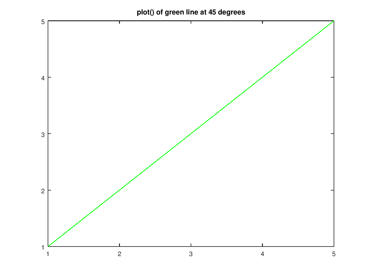
The following code
 x = 1:5;  y = 1:5;
 plot (x,y,"g");
 title ("plot() of green line at 45 degrees");
Produces the following figure
| Figure 1 |
|---|
 |
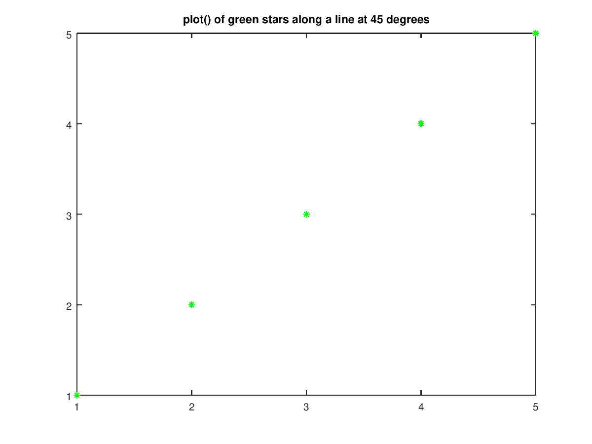
The following code
 x = 1:5;  y = 1:5;
 plot (x,y,"g*");
 title ("plot() of green stars along a line at 45 degrees");
Produces the following figure
| Figure 1 |
|---|
 |
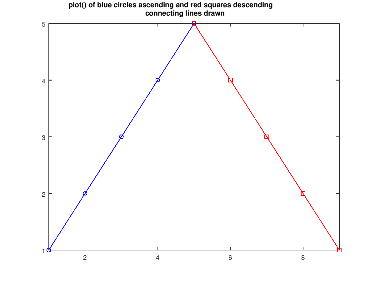
The following code
 x1 = 1:5;  y1 = 1:5;
 x2 = 5:9; y2 = 5:-1:1;
 plot (x1,y1,"bo-", x2,y2,"rs-");
 axis ("tight");
 title ({"plot() of blue circles ascending and red squares descending";
         "connecting lines drawn"});
Produces the following figure
| Figure 1 |
|---|
 |
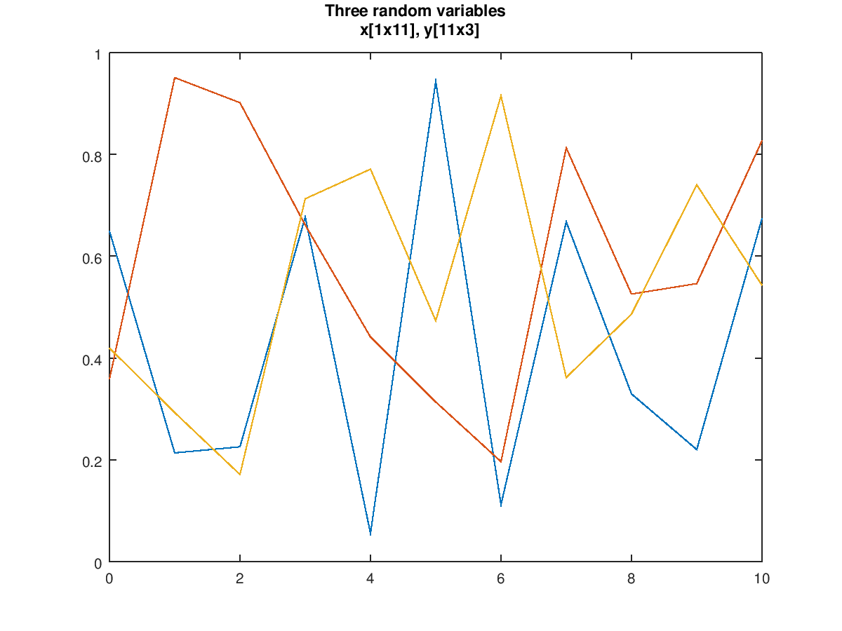
The following code
 x = 0:10;
 plot (x, rand (numel (x), 3));
 axis ([0 10 0 1]);
 title ({"Three random variables", "x[1x11], y[11x3]"});
Produces the following figure
| Figure 1 |
|---|
 |
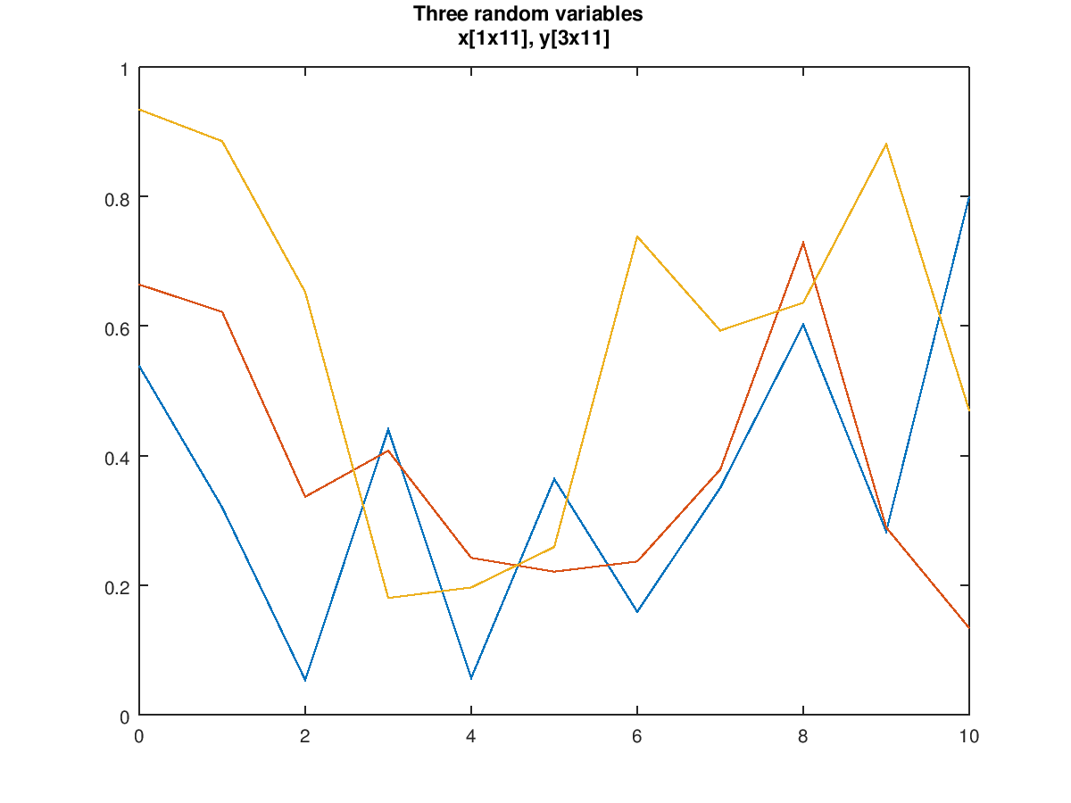
The following code
 x = 0:10;
 plot (x, rand (3, numel (x)));
 axis ([0 10 0 1]);
 title ({"Three random variables", "x[1x11], y[3x11]"});
Produces the following figure
| Figure 1 |
|---|
 |
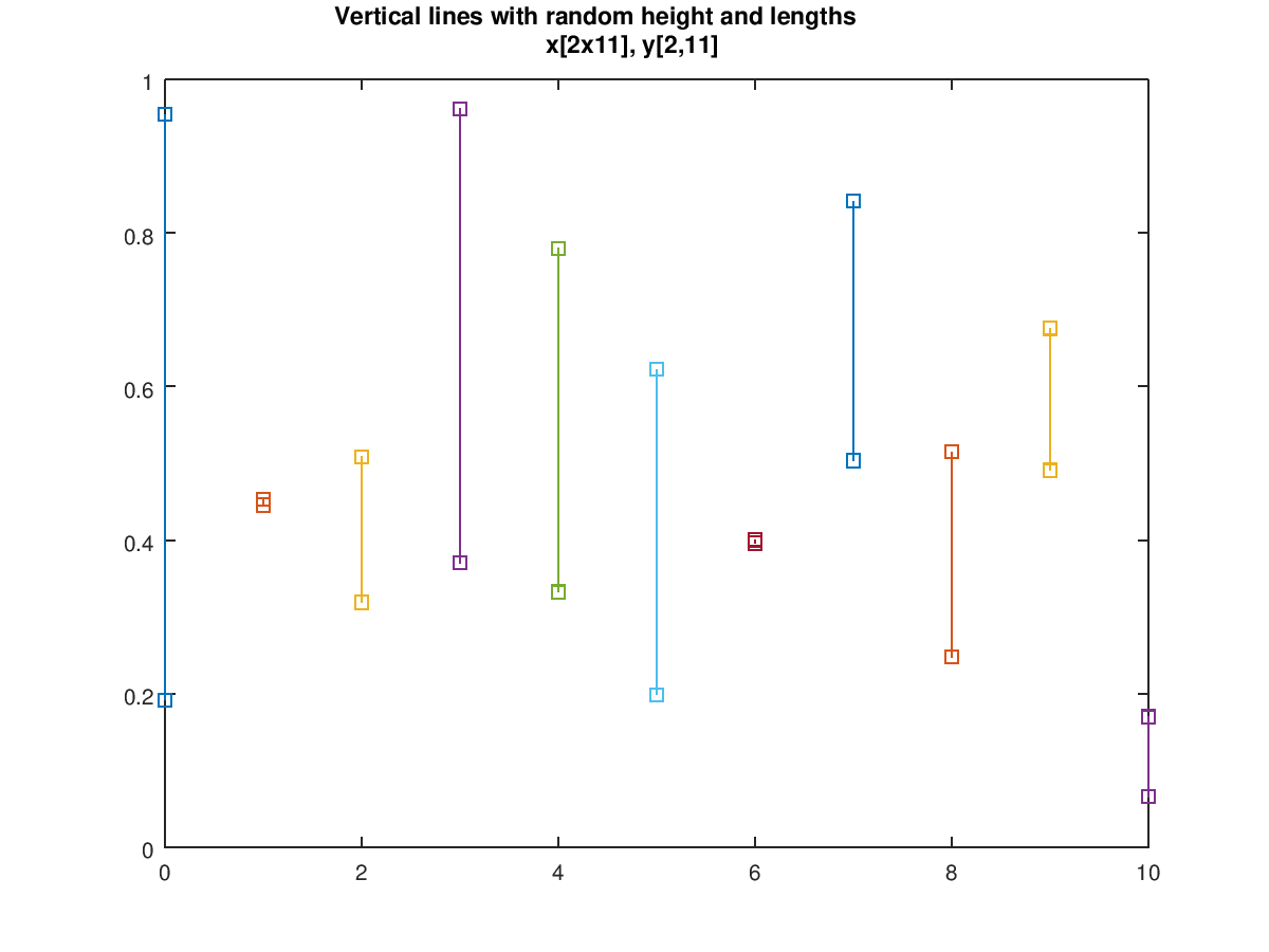
The following code
 x = 0:10;
 plot (repmat (x, 2, 1), rand (2, numel (x)), "-s");
 axis ([0 10 0 1]);
 title ({"Vertical lines with random height and lengths", ...
         "x[2x11], y[2,11]"});
Produces the following figure
| Figure 1 |
|---|
 |
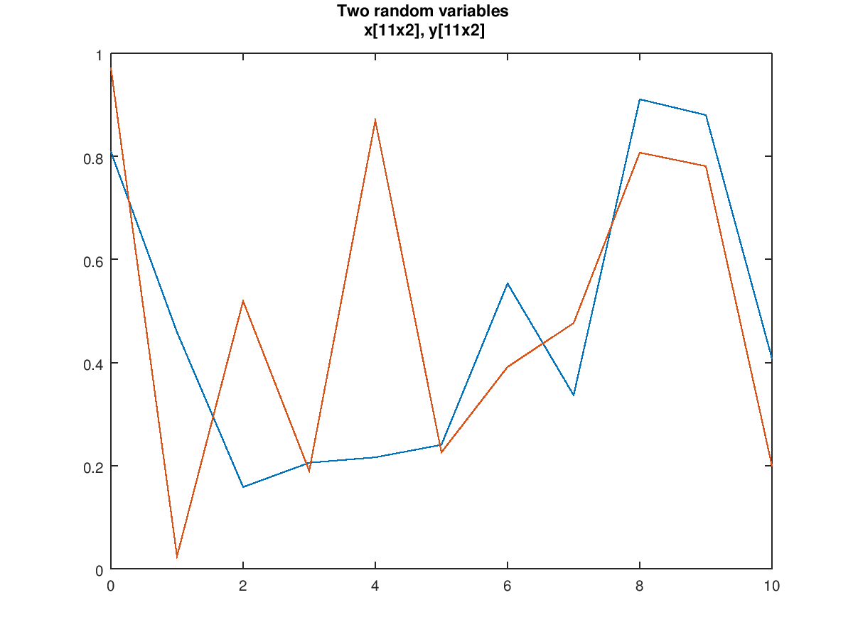
The following code
 x = 0:10;
 plot (repmat (x(:), 1, 2), rand (numel (x), 2));
 axis ([0 10 0 1]);
 title ({"Two random variables", "x[11x2], y[11x2]"});
Produces the following figure
| Figure 1 |
|---|
 |
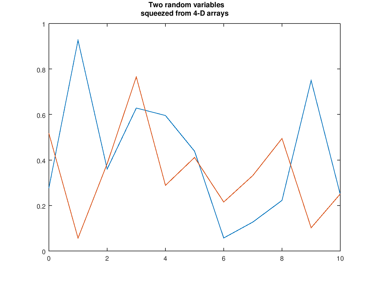
The following code
 x = 0:10;
 shape = [1, 1, numel(x), 2];
 x = reshape (repmat (x(:), 1, 2), shape);
 y = rand (shape);
 plot (x, y);
 axis ([0 10 0 1]);
 title ({"Two random variables", "squeezed from 4-D arrays"});
Produces the following figure
| Figure 1 |
|---|
 |
Package: octave