
|
Octave-Forge - Extra packages for GNU Octave |
| Home · Packages · Developers · Documentation · FAQ · Bugs · Mailing Lists · Links · Code |
|
|
Octave-Forge - Extra packages for GNU Octave |
| Home · Packages · Developers · Documentation · FAQ · Bugs · Mailing Lists · Links · Code |
Produce 3-D plots.
Many different combinations of arguments are possible. The simplest form is
plot3 (x, y, z)
in which the arguments are taken to be the vertices of the points to be plotted in three dimensions. If all arguments are vectors of the same length, then a single continuous line is drawn. If all arguments are matrices, then each column of is treated as a separate line. No attempt is made to transpose the arguments to make the number of rows match.
If only two arguments are given, as
plot3 (x, cplx)
the real and imaginary parts of the second argument are used as the y and z coordinates, respectively.
If only one argument is given, as
plot3 (cplx)
the real and imaginary parts of the argument are used as the y and z values, and they are plotted versus their index.
Arguments may also be given in groups of three as
plot3 (x1, y1, z1, x2, y2, z2, …)
in which each set of three arguments is treated as a separate line or set of lines in three dimensions.
To plot multiple one- or two-argument groups, separate each group with an empty format string, as
plot3 (x1, c1, "", c2, "", …)
Multiple property-value pairs may be specified which will affect the line
objects drawn by plot3. If the fmt argument is supplied it
will format the line objects in the same manner as plot.
If the first argument hax is an axes handle, then plot into this axis,
rather than the current axes returned by gca.
The optional return value h is a graphics handle to the created plot.
Example:
z = [0:0.05:5];
plot3 (cos (2*pi*z), sin (2*pi*z), z, ";helix;");
plot3 (z, exp (2i*pi*z), ";complex sinusoid;");
See also: ezplot3, plot.
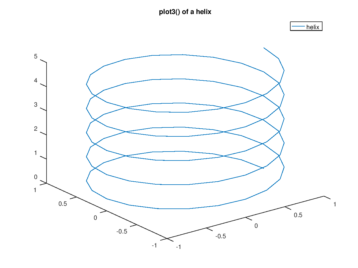
The following code
 clf;
 z = [0:0.05:5];
 plot3 (cos (2*pi*z), sin (2*pi*z), z);
 legend ("helix");
 title ("plot3() of a helix");
Produces the following figure
| Figure 1 |
|---|
 |
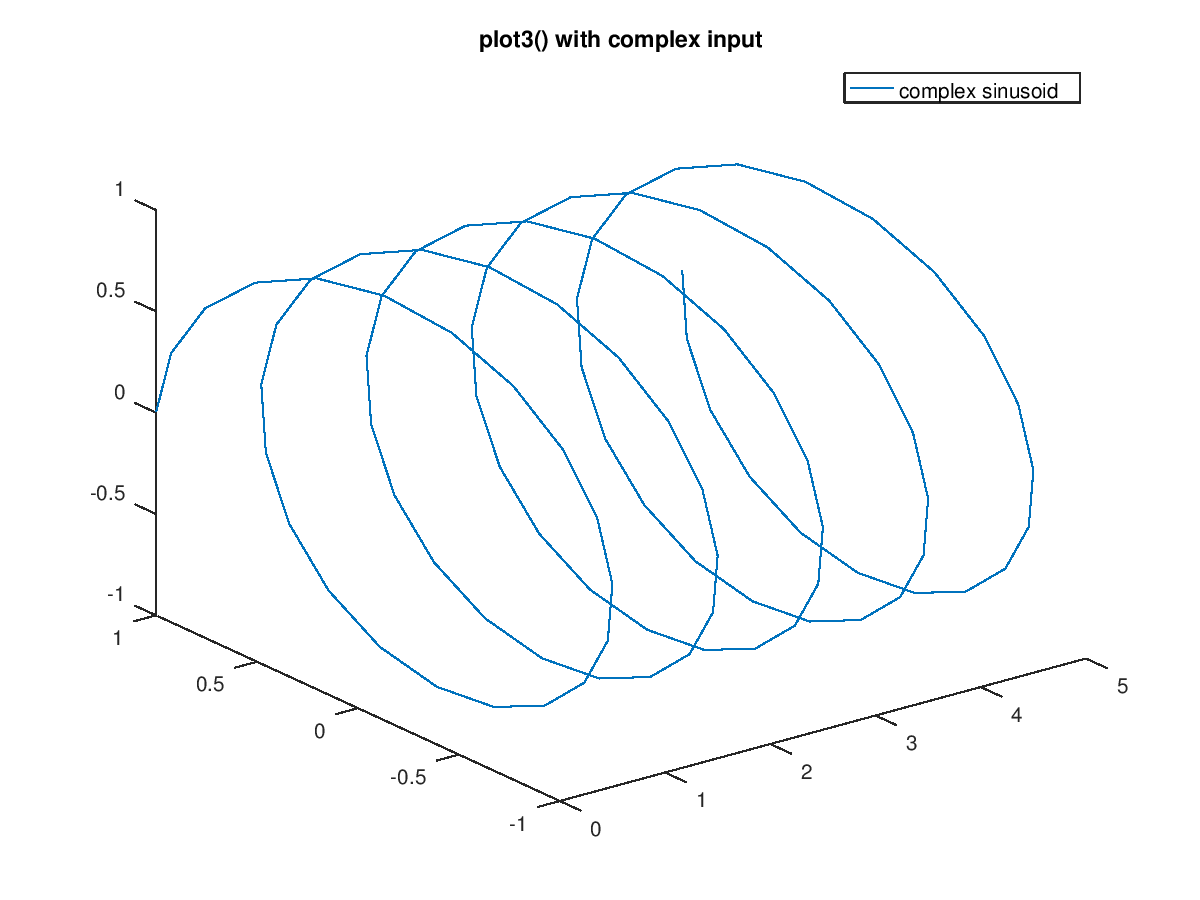
The following code
 clf;
 z = [0:0.05:5];
 plot3 (z, exp (2i*pi*z));
 legend ("complex sinusoid");
 title ("plot3() with complex input");
Produces the following figure
| Figure 1 |
|---|
 |
Package: octave