|
Octave-Forge - Extra packages for GNU Octave |
| Home · Packages · Developers · Documentation · FAQ · Bugs · Mailing Lists · Links · Code |
Plot a 2-D vector field with arrows.
Plot the (u, v) components of a vector field in an (x, y) meshgrid. If the grid is uniform then x and y can be specified as vectors.
If x and y are undefined they are assumed to be
(1:m, 1:n) where
[m, n] = size (u).
The variable s is a scalar defining a scaling factor to use for the arrows of the field relative to the mesh spacing. A value of 0 disables all scaling. The default value is 0.9.
The style to use for the plot can be defined with a line style style
of the same format as the plot command.
If a marker is specified then markers at the grid points of the vectors are
drawn rather than arrows. If the argument "filled" is given then
the markers are filled.
If the first argument hax is an axes handle, then plot into this axis,
rather than the current axes returned by gca.
The optional return value h is a graphics handle to a quiver object. A quiver object regroups the components of the quiver plot (body, arrow, and marker), and allows them to be changed together.
Example:
[x, y] = meshgrid (1:2:20);
h = quiver (x, y, sin (2*pi*x/10), sin (2*pi*y/10));
set (h, "maxheadsize", 0.33);
See also: quiver3, compass, feather, plot.
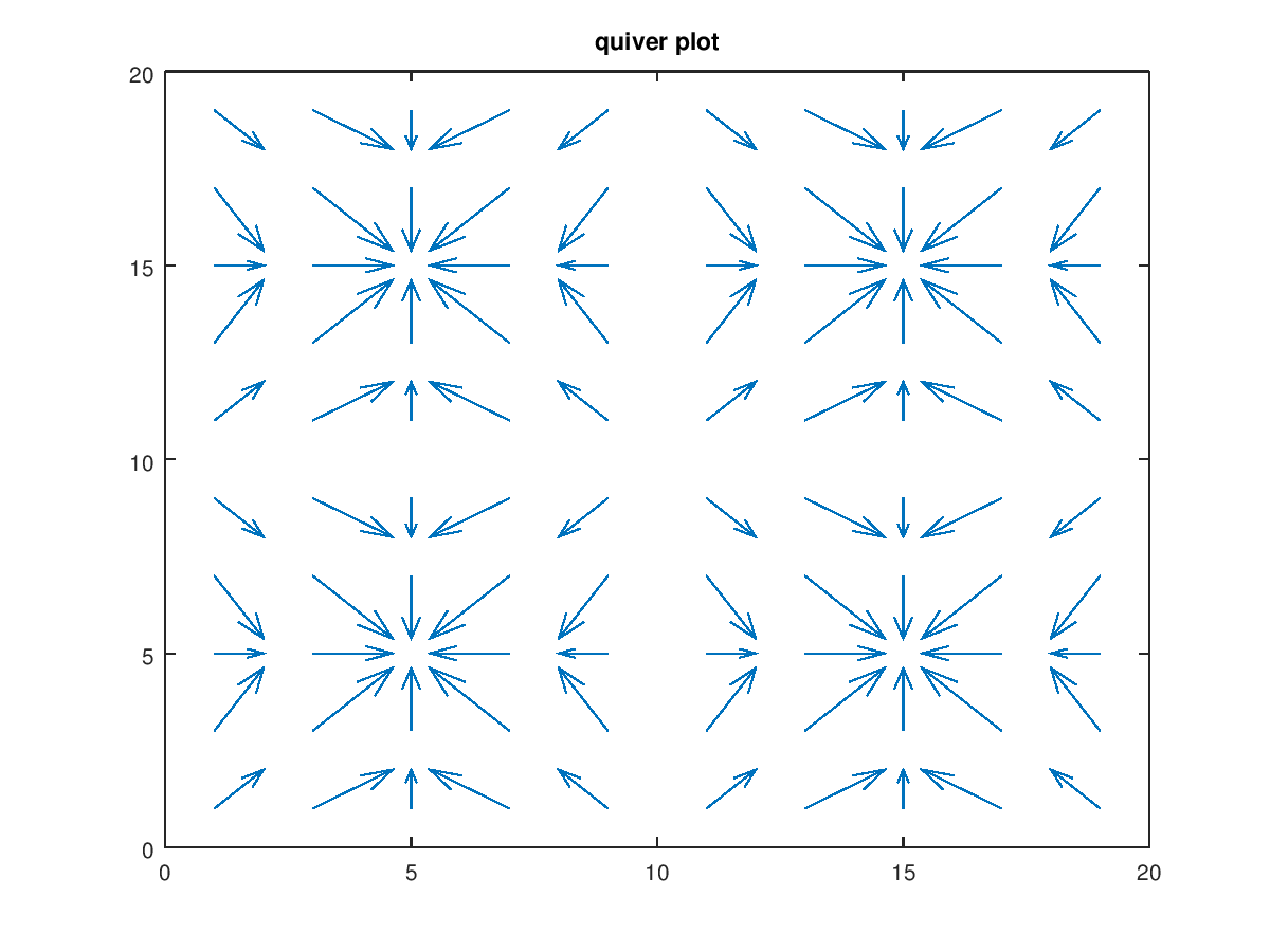
The following code
 clf;
 [x,y] = meshgrid (1:2:20);
 h = quiver (x,y, sin (2*pi*x/10), sin (2*pi*y/10));
 title ("quiver plot");
Produces the following figure
| Figure 1 |
|---|
 |
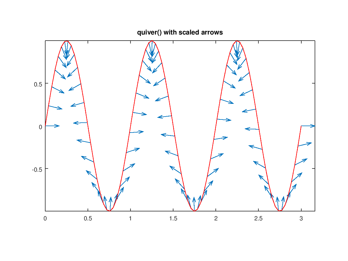
The following code
 clf;
 x = linspace (0, 3, 80);
 y = sin (2*pi*x);
 theta = 2*pi*x + pi/2;
 quiver (x, y, sin (theta)/10, cos (theta)/10, 0.4);
 axis equal tight;
 hold on; plot (x,y,"r"); hold off;
 title ("quiver() with scaled arrows");
Produces the following figure
| Figure 1 |
|---|
 |
Package: octave