
|
Octave-Forge - Extra packages for GNU Octave |
| Home · Packages · Developers · Documentation · FAQ · Bugs · Mailing Lists · Links · Code |
|
|
Octave-Forge - Extra packages for GNU Octave |
| Home · Packages · Developers · Documentation · FAQ · Bugs · Mailing Lists · Links · Code |
Fit a piecewise cubic spline with breaks (knots) breaks to the noisy data, x and y.
x is a vector, and y is a vector or N-D array. If y is an N-D array, then x(j) is matched to y(:,…,:,j).
p is a positive integer defining the number of intervals along x, and p+1 is the number of breaks. The number of points in each interval differ by no more than 1.
The optional property periodic is a logical value which specifies
whether a periodic boundary condition is applied to the spline. The
length of the period is max (breaks) - min (breaks).
The default value is false.
The optional property robust is a logical value which specifies if robust fitting is to be applied to reduce the influence of outlying data points. Three iterations of weighted least squares are performed. Weights are computed from previous residuals. The sensitivity of outlier identification is controlled by the property beta. The value of beta is restricted to the range, 0 < beta < 1. The default value is beta = 1/2. Values close to 0 give all data equal weighting. Increasing values of beta reduce the influence of outlying data. Values close to unity may cause instability or rank deficiency.
The fitted spline is returned as a piecewise polynomial, pp, and
may be evaluated using ppval.
The splines are constructed of polynomials with degree order. The default is a cubic, order=3. A spline with P pieces has P+order degrees of freedom. With periodic boundary conditions the degrees of freedom are reduced to P.
The optional property, constaints, is a structure specifying linear
constraints on the fit. The structure has three fields, "xc",
"yc", and "cc".
"xc"Vector of the x-locations of the constraints.
"yc"Constraining values at the locations xc. The default is an array of zeros.
"cc"Coefficients (matrix). The default is an array of ones. The number of rows is limited to the order of the piecewise polynomials, order.
Constraints are linear combinations of derivatives of order 0 to order-1 according to
cc(1,j) * y(xc(j)) + cc(2,j) * y'(xc(j)) + ... = yc(:,...,:,j).
See also: interp1, unmkpp, ppval, spline, pchip, ppder, ppint, ppjumps.
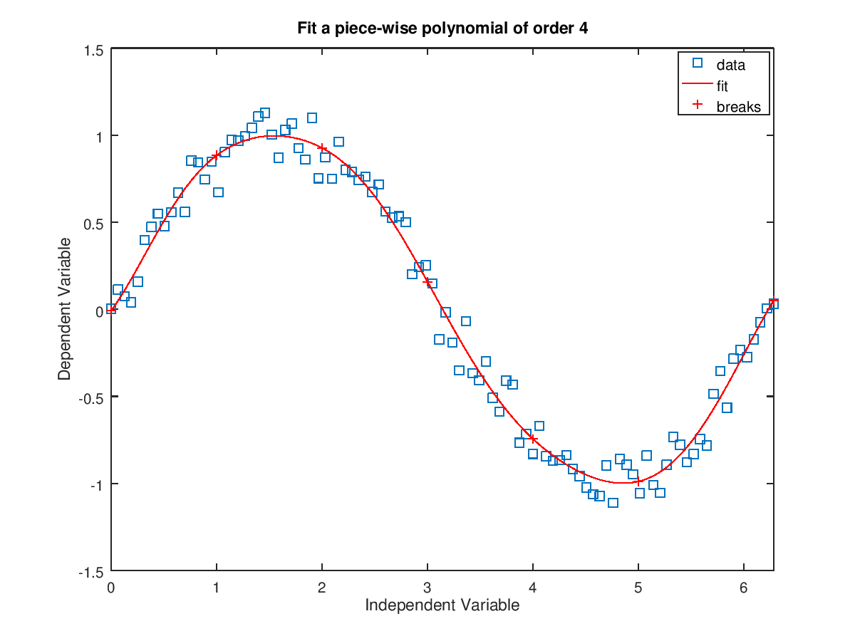
The following code
 % Noisy data
 x = linspace (0, 2*pi, 100);
 y = sin (x) + 0.1 * randn (size (x));
 % Breaks
 breaks = [0:5, 2*pi];
 % Fit a spline of order 5
 pp = splinefit (x, y, breaks, "order", 4);
 clf;
 plot (x, y, "s", x, ppval (pp, x), "r", breaks, ppval (pp, breaks), "+r");
 xlabel ("Independent Variable");
 ylabel ("Dependent Variable");
 title ("Fit a piece-wise polynomial of order 4");
 legend ({"data", "fit", "breaks"});
 axis tight
 ylim auto
Produces the following figure
| Figure 1 |
|---|
 |
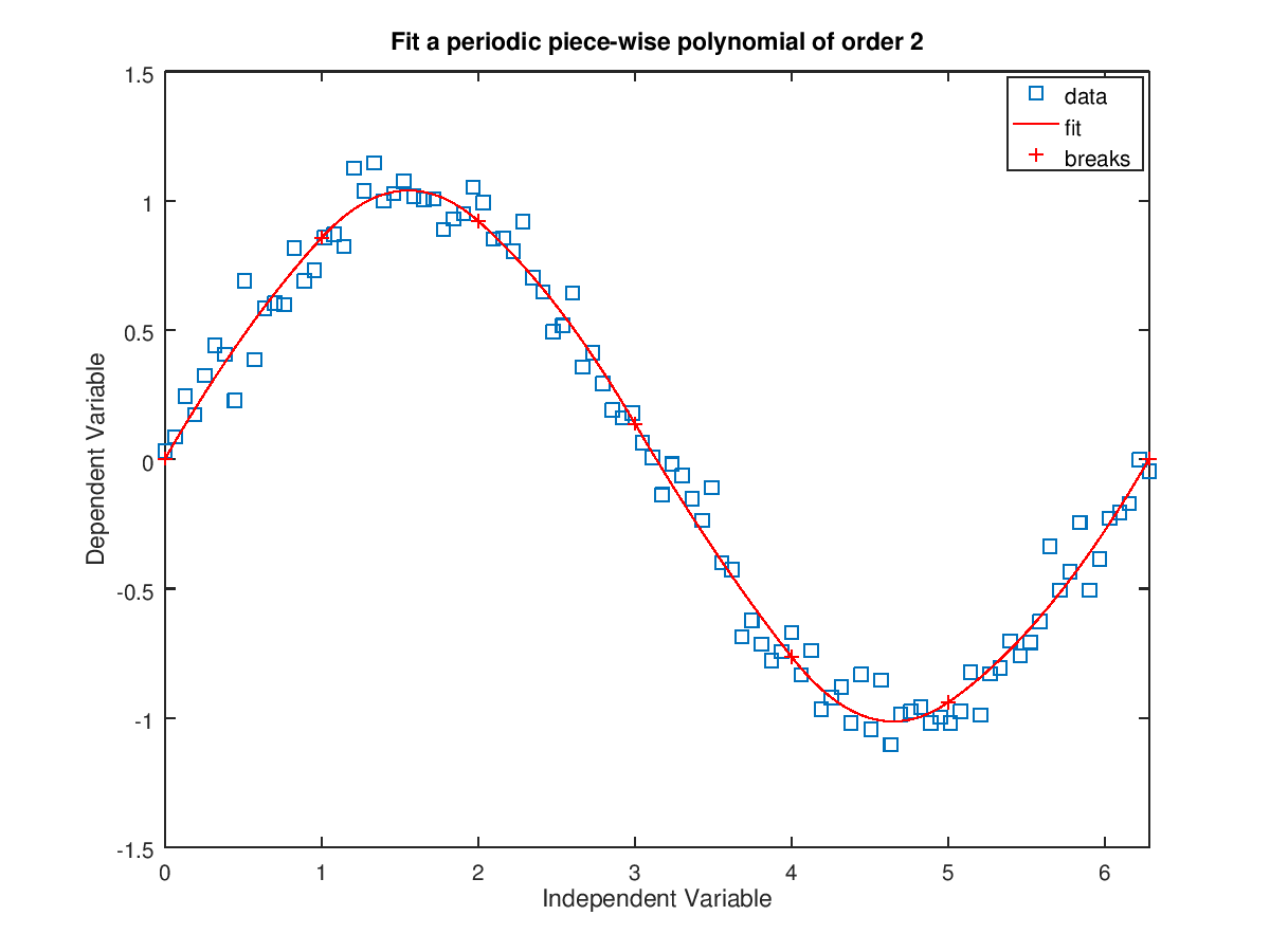
The following code
 % Noisy data
 x = linspace (0,2*pi, 100);
 y = sin (x) + 0.1 * randn (size (x));
 % Breaks
 breaks = [0:5, 2*pi];
 % Fit a spline of order 3 with periodic boundary conditions
 pp = splinefit (x, y, breaks, "order", 2, "periodic", true);
 clf;
 plot (x, y, "s", x, ppval (pp, x), "r", breaks, ppval (pp, breaks), "+r");
 xlabel ("Independent Variable");
 ylabel ("Dependent Variable");
 title ("Fit a periodic piece-wise polynomial of order 2");
 legend ({"data", "fit", "breaks"});
 axis tight
 ylim auto
Produces the following figure
| Figure 1 |
|---|
 |
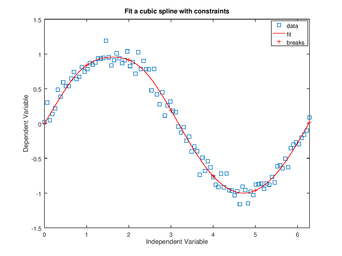
The following code
 % Noisy data
 x = linspace (0, 2*pi, 100);
 y = sin (x) + 0.1 * randn (size (x));
 % Breaks
 breaks = [0:5, 2*pi];
 % Constraints: y(0) = 0, y'(0) = 1 and y(3) + y"(3) = 0
 xc = [0 0 3];
 yc = [0 1 0];
 cc = [1 0 1; 0 1 0; 0 0 1];
 con = struct ("xc", xc, "yc", yc, "cc", cc);
 % Fit a cubic spline with 8 pieces and constraints
 pp = splinefit (x, y, 8, "constraints", con);
 clf;
 plot (x, y, "s", x, ppval (pp, x), "r", breaks, ppval (pp, breaks), "+r");
 xlabel ("Independent Variable");
 ylabel ("Dependent Variable");
 title ("Fit a cubic spline with constraints");
 legend ({"data", "fit", "breaks"});
 axis tight
 ylim auto
Produces the following figure
| Figure 1 |
|---|
 |
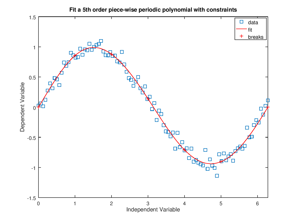
The following code
 % Noisy data
 x = linspace (0, 2*pi, 100);
 y = sin (x) + 0.1 * randn (size (x));
 % Breaks
 breaks = [0:5, 2*pi];
 xc = [0 0 3];
 yc = [0 1 0];
 cc = [1 0 1; 0 1 0; 0 0 1];
 con = struct ("xc", xc, "yc", yc, "cc", cc);
 % Fit a spline of order 6 with constraints and periodicity
 pp = splinefit (x, y, breaks, "constraints", con, "order", 5, "periodic", true);
 clf;
 plot (x, y, "s", x, ppval (pp, x), "r", breaks, ppval (pp, breaks), "+r");
 xlabel ("Independent Variable");
 ylabel ("Dependent Variable");
 title ("Fit a 5th order piece-wise periodic polynomial with constraints");
 legend ({"data", "fit", "breaks"});
 axis tight
 ylim auto
Produces the following figure
| Figure 1 |
|---|
 |
Package: octave