Function Reference: @abcd/trace

Function File: rout = trace(abcd, rin, do_plot): Trace the rays rin through abcd. If do_plot is true, create also a plot with the trace.

Demonstration 1

The following code

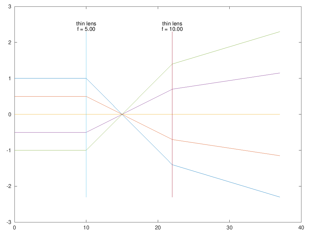
 s = abcd ("propagation", 10,
           "thin-lens", 5,
           "propagation", 12,
           "thin-lens", 10,
           "propagation", 15);

 rin = [1 0.5 0 -0.5 -1; 0 0 0 0 0];
 rout = trace(s, rin, true)

Produces the following output

rout =

  -2.30000  -1.15000   0.00000   1.15000   2.30000
  -0.06000  -0.03000   0.00000   0.03000   0.06000

and the following figure

Figure 1

Demonstration 2

The following code

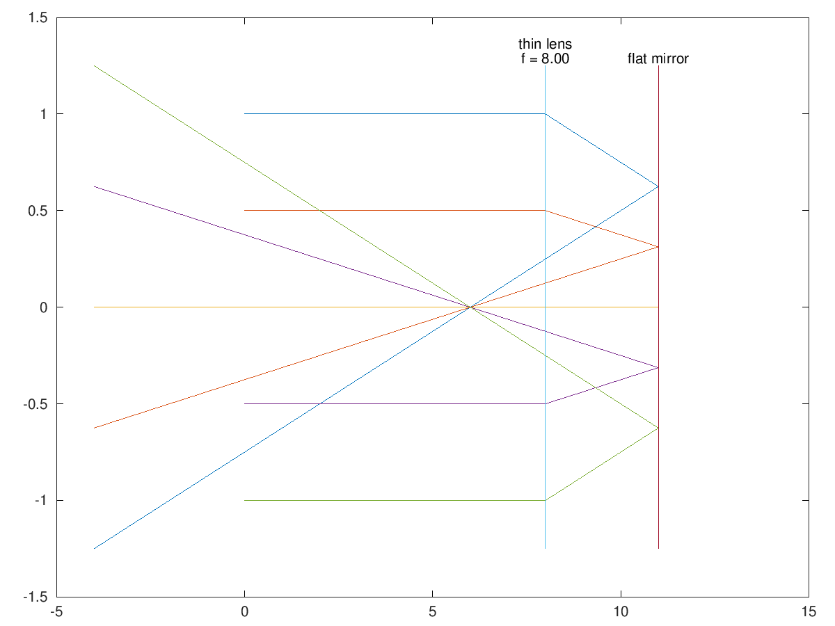
 s = abcd ("propagation", 8,
           "thin-lens", 8,
           "propagation", 3,
           "flat-mirror", [],
           "propagation", 15);

 rin = [1 0.5 0 -0.5 -1; 0 0 0 0 0];
 rout = trace(s, rin, true)

Produces the following output

rout =

  -1.25000  -0.62500   0.00000   0.62500   1.25000
  -0.12500  -0.06250   0.00000   0.06250   0.12500

and the following figure

Figure 1

Demonstration 3

The following code

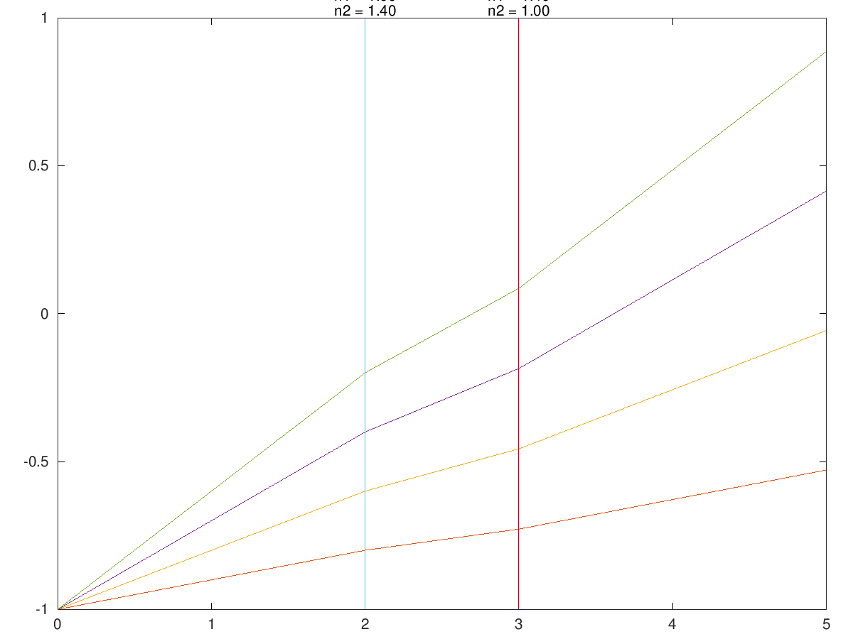
 s = abcd ("propagation", 2,
           "flat-refraction", [1, 1.4],
           "propagation", 1,
           "flat-refraction", [1.4, 1],
           "propagation", 2);

 rin = [-1 -1 -1 -1 -1; 0.0 0.1 0.2 0.3 0.4];
 rout = trace(s, rin, true)

Produces the following output

rout =

  -1.00000  -0.52857  -0.05714   0.41429   0.88571
   0.00000   0.10000   0.20000   0.30000   0.40000

and the following figure

Figure 1

Demonstration 4

The following code

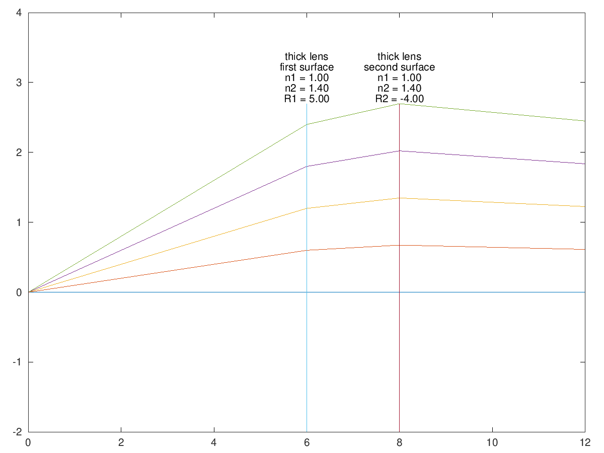
 s = abcd ("propagation", 6,
           "thick-lens", [1, 1.4, 5, -4, 2],
           "propagation", 4);

 rin = [0 0 0 0 0; 0.0 0.1 0.2 0.3 0.4];
 rout = trace(s, rin, true)
 axis([0 12 -2 4])

Produces the following output

rout =

   0.00000   0.61257   1.22514   1.83771   2.45029
   0.00000  -0.01543  -0.03086  -0.04629  -0.06171

and the following figure

Figure 1

Package: optics