- Function File: LinearRegression
(F, y)¶ - Function File: LinearRegression
(F, y, w)¶ - Function File:
[p, e_var, r, p_var, fit_var] =LinearRegression(…)¶ -
general linear regression
determine the parameters p_j (j=1,2,...,m) such that the function f(x) = sum_(j=1,...,m) p_j*f_j(x) is the best fit to the given values y_i by f(x_i) for i=1,...,n, i.e. minimize sum_(i=1,...,n)(y_i-sum_(j=1,...,m) p_j*f_j(x_i))^2 with respect to p_j
parameters:
- F is an n*m matrix with the values of the basis functions at the support points. In column j give the values of f_j at the points x_i (i=1,2,...,n)
- y is a column vector of length n with the given values
- w is a column vector of length n with the weights of the data points. 1/w_i is expected to be proportional to the estimated uncertainty in the y values. Then the weighted expression sum_(i=1,...,n)(w_i^2*(y_i-f(x_i))^2) is minimized.
return values:
- p is the vector of length m with the estimated values of the parameters
- e_var is the vector of estimated variances of the provided y values. If weights are provided, then the product e_var_i * w^2_i is assumed to be constant.
- r is the weighted norm of the residual
- p_var is the vector of estimated variances of the parameters p_j
- fit_var is the vector of the estimated variances of the fitted function values f(x_i)
To estimate the variance of the difference between future y values and fitted y values use the sum of e_var and fit_var
Caution: do NOT request fit_var for large data sets, as a n by n matrix is generated
See also: ols,gls,regress,leasqr,nonlin_curvefit,polyfit,wpolyfit,expfit.
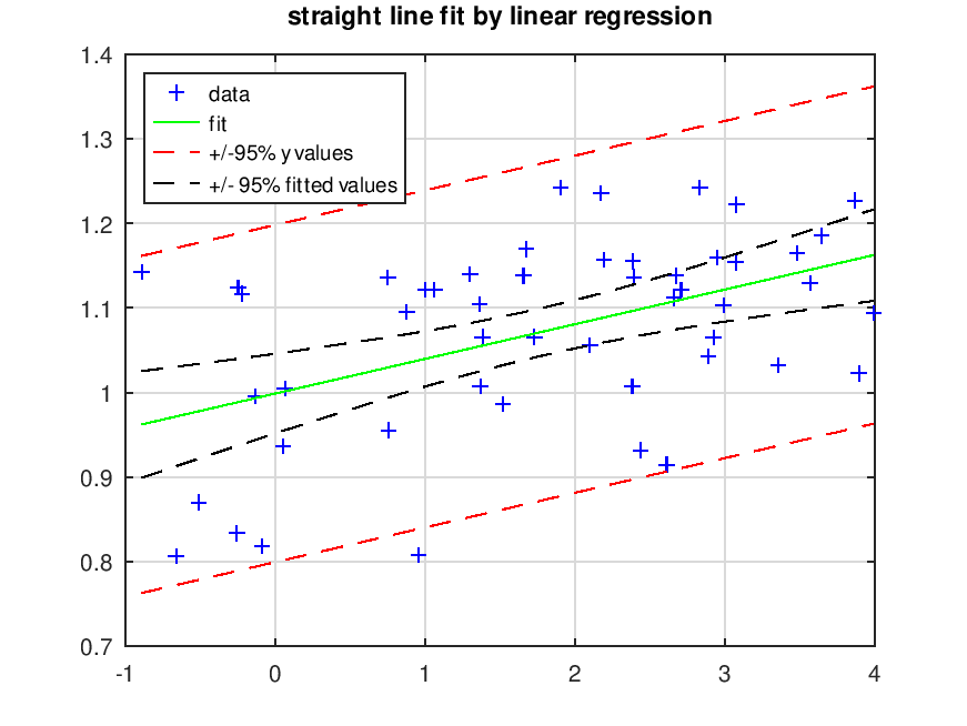
Demonstration 1
The following code
 n = 50;
 x = sort (rand (n,1) * 5 - 1);
 y = 1 + 0.05 * x + 0.1 * randn (size (x));
 F = [ones(n, 1), x(:)];
 [p, e_var, r, p_var, fit_var] = LinearRegression (F, y);
 yFit = F * p;
 figure ()
 plot(x, y, '+b', x, yFit, '-g',...
      x, yFit + 1.96 * sqrt (e_var), '--r',...
      x, yFit + 1.96 * sqrt (fit_var), '--k',...
      x, yFit - 1.96 * sqrt (e_var), '--r',...
      x, yFit - 1.96 * sqrt (fit_var), '--k')
 title ('straight line fit by linear regression')
 legend ('data','fit','+/-95% y values','+/- 95% fitted values','location','northwest')
 grid on
Produces the following figure
| Figure 1 |
|---|
 |
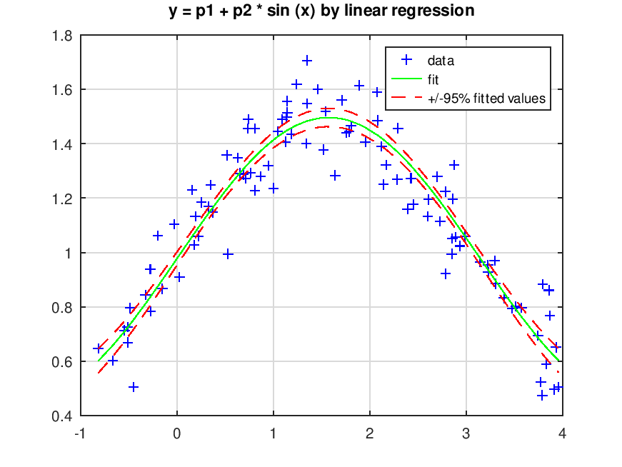
Demonstration 2
The following code
 n = 100;
 x = sort (rand (n, 1) * 5 - 1);
 y = 1 + 0.5 * sin (x) + 0.1 * randn (size (x));
 F = [ones(n, 1), sin(x(:))];
 [p, e_var, r, p_var, fit_var] = LinearRegression (F, y);
 yFit = F * p;
 figure ()
 plot (x, y, '+b', x, yFit, '-g', x, yFit + 1.96 * sqrt (fit_var),
       '--r', x, yFit - 1.96 * sqrt (fit_var), '--r')
 title ('y = p1 + p2 * sin (x) by linear regression')
 legend ('data', 'fit', '+/-95% fitted values')
 grid on
Produces the following figure
| Figure 1 |
|---|
 |
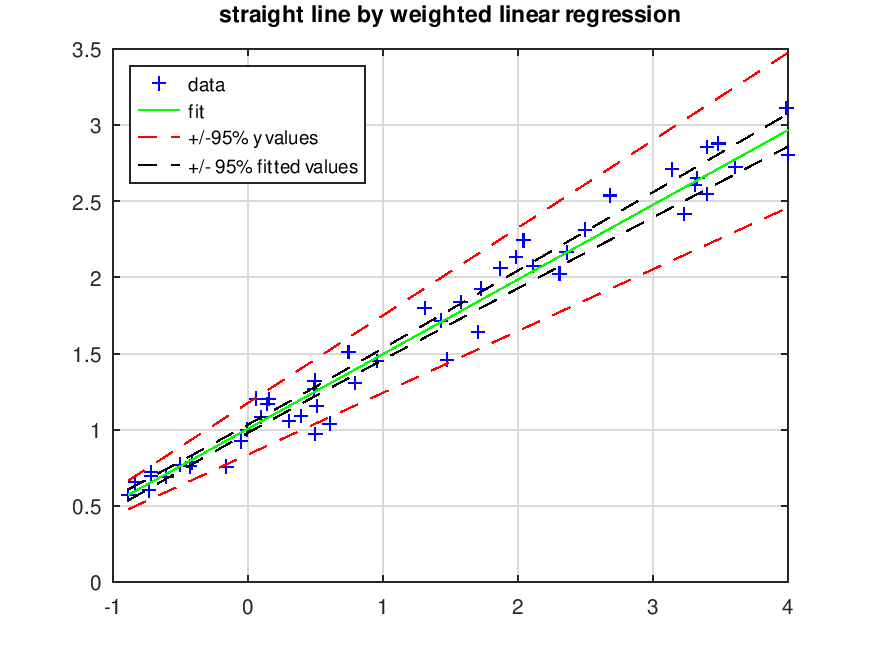
Demonstration 3
The following code
 n = 50;
 x = sort (rand (n, 1) * 5 - 1);
 y = 1 + 0.5 * x;
 dy = 1 ./ y;  # constant relative error is assumed
 y = y + 0.1 * randn (size (x)) .* y;  # straight line with relative size noise
 F = [ones(n, 1), x(:)];
 [p, e_var, r, p_var, fit_var] = LinearRegression (F, y, dy); # weighted regression
 fitted_parameters_and_StdErr = [p, sqrt(p_var)]
 yFit = F * p;
 figure ()
 plot(x, y, '+b', x, yFit, '-g',...
      x, yFit + 1.96 * sqrt (e_var), '--r',...
      x, yFit + 1.96 * sqrt (fit_var), '--k',...
      x, yFit - 1.96 * sqrt (e_var), '--r',...
      x, yFit - 1.96 * sqrt (fit_var), '--k')
 title ('straight line by weighted linear regression')
 legend ('data','fit','+/-95% y values','+/- 95% fitted values','location','northwest')
 grid on
Produces the following output
fitted_parameters_and_StdErr =

   1.021554   0.020916
   0.464942   0.016079
and the following figure
| Figure 1 |
|---|
 |
Package: optim