USAGE  [alpha,c,rms] = pronyfit( deg, x1, h, y )

 Prony's method for non-linear exponential fitting

 Fit function:   \sum_1^{deg} c(i)*exp(alpha(i)*x)

 Elements of data vector y must correspond to
 equidistant x-values starting at x1 with stepsize h

 The method is fully compatible with complex linear
 coefficients c, complex nonlinear coefficients alpha
 and complex input arguments y, x1, non-zero h .
 Fit-order deg  must be a real positive integer.

 Returns linear coefficients c, nonlinear coefficients
 alpha and root mean square error rms. This method is
 known to be more stable than 'brute-force' non-linear
 least squares fitting.

 Example
    x0 = 0; step = 0.05; xend = 5; x = x0:step:xend;
    y = 2*exp(1.3*x)-0.5*exp(2*x);
    error = (rand(1,length(y))-0.5)*1e-4;
    [alpha,c,rms] = pronyfit(2,x0,step,y+error)

  alpha =
    2.0000
    1.3000
  c =
    -0.50000
     2.00000
  rms = 0.00028461

 The fit is very sensitive to the number of data points.
 It doesn't perform very well for small data sets.
 Theoretically, you need at least 2*deg data points, but
 if there are errors on the data, you certainly need more.

 Be aware that this is a very (very,very) ill-posed problem.
 By the way, this algorithm relies heavily on computing the
 roots of a polynomial. I used 'roots.m', if there is
 something better please use that code.

 Demo for a complex fit-function:
 deg= 2; N= 20; x1= -(1+i), x= linspace(x1,1+i/2,N).';
 h = x(2) - x(1)
 y= (2+i)*exp( (-1-2i)*x ) + (-1+3i)*exp( (2+3i)*x );
 A= 5e-2; y+= A*(randn(N,1)+randn(N,1)*i); % add complex noise
 [alpha,c,rms]= pronyfit( deg, x1, h, y )

Demonstration 1

	 % same as in help - part
 deg= 2; N= 20; x1= -(1+i), x= linspace(x1,1+i/2,N).';
 h = x(2) - x(1)
 y= (2+i)*exp( (-1-2i)*x ) + (-1+3i)*exp( (2+3i)*x );
 A= 5e-2; y+= A*(randn(N,1)+randn(N,1)*i); % add complex noise
 [alpha,c,rms]= pronyfit( deg, x1, h, y )

x1 = -1 - 1i
h =  0.105263 + 0.078947i
alpha =

  -1.1732 - 1.9061i
   2.0068 + 2.9850i

c =

   2.0683 + 0.9808i
  -1.0138 + 3.0253i

rms = 0.8352

Demonstration 2

	 % demo for stepsize with negative real part
 deg= 2; N= 20; x1= +3*(1+i), x= linspace(x1,1+i/3,N).';
 h = x(2) - x(1)
 y= (2+i)*exp( (-1-2i)*x ) + (-1+3i)*exp( (2+3i)*x );
 A= 5e-2; y+= A*(randn(N,1)+randn(N,1)*i); % add complex noise
 [alpha,c,rms]= pronyfit( deg, x1, h, y )

x1 =  3 + 3i
h = -0.1053 - 0.1404i
alpha =

   2.0221 + 3.0103i
  -0.9970 - 1.9970i

c =

  -0.9080 + 2.9715i
   2.0140 + 0.9670i

rms = 0.3046

Demonstration 3

The following code

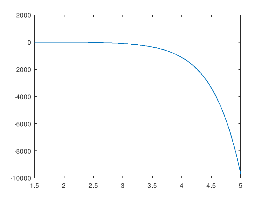
 x0 = 1.5; step = 0.05; xend = 5;
 a = [1.3, 2]';
 c = [2, -0.5]';
 v = 1e-4;
 
 x = x0:step:xend;
 y = exp (x(:) * a(:).') * c(:);
 err = randn (size (y)) * v;
 plot (x, y + err);
 
 [a_out, c_out, rms] = pronyfit (2, x0, step, y+err)

Produces the following output

a_out =

   2.0000
   1.3000

c_out =

  -0.5000
   2.0000

rms = 1.3873e-03

and the following figure

Figure 1

Package: optim