- Function File: p = ctmc (Q)
- Function File: p = ctmc (Q, t, p0)
-
Compute stationary or transient state occupancy probabilities for a continuous-time Markov chain.
With a single argument, compute the stationary state occupancy probabilities p(1), …, p(N) for a continuous-time Markov chain with finite state space {1, …, N} and N \times N infinitesimal generator matrix Q. With three arguments, compute the state occupancy probabilities p(1), …, p(N) that the system is in state i at time t, given initial state occupancy probabilities p0(1), …, p0(N) at time 0.
INPUTS
Q(i,j)Infinitesimal generator matrix. Q is a N \times N square matrix where
Q(i,j)is the transition rate from state i to state j, for 1 ≤ i \neq j ≤ N. Q must satisfy the property that \sum_{j=1}^N Q_{i, j} = 0tTime at which to compute the transient probability (t ≥ 0). If omitted, the function computes the steady state occupancy probability vector.
p0(i)probability that the system is in state i at time 0.
OUTPUTS
p(i)If this function is invoked with a single argument,
p(i)is the steady-state probability that the system is in state i, i = 1, …, N. If this function is invoked with three arguments,p(i)is the probability that the system is in state i at time t, given the initial occupancy probabilities p0(1), …, p0(N).
See also: dtmc.
Demonstration 1
The following code
 Q = [ -1  1; ...
        1 -1  ];
 q = ctmc(Q)
Produces the following output
q =

   0.50000   0.50000
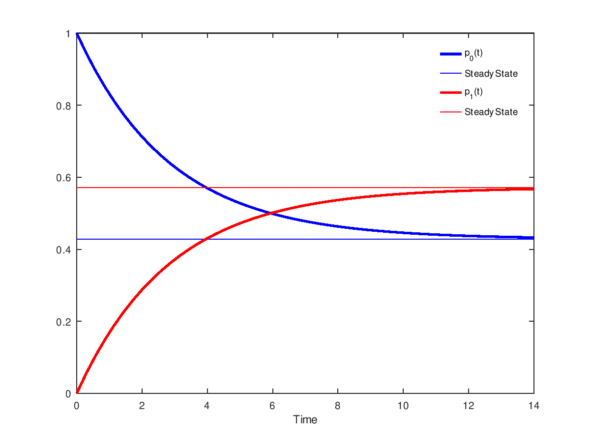
Demonstration 2
The following code
 a = 0.2;
 b = 0.15;
 Q = [ -a a; b -b];
 T = linspace(0,14,50);
 pp = zeros(2,length(T));
 for i=1:length(T)
   pp(:,i) = ctmc(Q,T(i),[1 0]);
 endfor
 ss = ctmc(Q); # compute steady state probabilities
 plot( T, pp(1,:), "b;p_0(t);", "linewidth", 2, ...
       T, ss(1)*ones(size(T)), "b;Steady State;", ...
       T, pp(2,:), "r;p_1(t);", "linewidth", 2, ...
       T, ss(2)*ones(size(T)), "r;Steady State;" );
 xlabel("Time");
 legend("boxoff");
Produces the following figure
q =

   0.50000   0.50000
| Figure 1 |
|---|
 |
Demonstration 3
The following code
 sec  = 1;
 min  = 60*sec;
 hour = 60*min;
 day  = 24*hour;
 year = 365*day;
 # state space enumeration {2, RC, RB, 1, 0}
 a = 1/(10*min);    # 1/a = duration of reboot (10 min)
 b = 1/(30*sec);    # 1/b = reconfiguration time (30 sec)
 g = 1/(5000*hour); # 1/g = processor MTTF (5000 hours)
 d = 1/(4*hour);    # 1/d = processor MTTR (4 hours)
 c = 0.9;           # coverage
 Q = [ -2*g 2*c*g 2*(1-c)*g      0  0; ...
          0    -b         0      b  0; ...
          0     0        -a      a  0; ...
          d     0         0 -(g+d)  g; ...
          0     0         0      d -d];
 p = ctmc(Q);
 A = p(1) + p(4);
 printf("System availability   %9.2f min/year\n",A*year/min);
 printf("Mean time in RB state %9.2f min/year\n",p(3)*year/min);
 printf("Mean time in RC state %9.2f min/year\n",p(2)*year/min);
 printf("Mean time in 0 state  %9.2f min/year\n",p(5)*year/min);
 Q(3,:) = Q(5,:) = 0; # make states 3 and 5 absorbing
 p0 = [1 0 0 0 0];
 MTBF = ctmcmtta(Q, p0) / hour;
 printf("System MTBF %.2f hours\n",MTBF);
Produces the following output
System availability   525594.26 min/year
Mean time in RB state      3.50 min/year
Mean time in RC state      1.57 min/year
Mean time in 0 state       0.67 min/year
System MTBF 24857.22 hours
| Figure 1 |
|---|
|
Package: queueing