Function File: p = dtmc (P)

Function File: p = dtmc (P, n, p0)

Compute stationary or transient state occupancy probabilities for a discrete-time Markov chain.

With a single argument, compute the stationary state occupancy probabilities p(1), …, p(N) for a discrete-time Markov chain with finite state space {1, …, N} and with N \times N transition matrix P. With three arguments, compute the transient state occupancy probabilities p(1), …, p(N) that the system is in state i after n steps, given initial occupancy probabilities p0(1), …, p0(N).

INPUTS

P(i,j)

transition probabilities from state i to state j. P must be an N \times N irreducible stochastic matrix, meaning that the sum of each row must be 1 (\sum_{j=1}^N P_{i, j} = 1), and the rank of P must be N.

n

Number of transitions after which state occupancy probabilities are computed (scalar, n ≥ 0)

p0(i)

probability that at step 0 the system is in state i (vector of length N).

OUTPUTS

p(i)

If this function is called with a single argument, p(i) is the steady-state probability that the system is in state i. If this function is called with three arguments, p(i) is the probability that the system is in state i after n transitions, given the probabilities p0(i) that the initial state is i.

See also: ctmc.

Demonstration 1

 P = zeros(9,9);
 P(1,[2 4]    ) = 1/2;
 P(2,[1 5 3]  ) = 1/3;
 P(3,[2 6]    ) = 1/2;
 P(4,[1 5 7]  ) = 1/3;
 P(5,[2 4 6 8]) = 1/4;
 P(6,[3 5 9]  ) = 1/3;
 P(7,[4 8]    ) = 1/2;
 P(8,[7 5 9]  ) = 1/3;
 P(9,[6 8]    ) = 1/2;
 p = dtmc(P);
 disp(p)

Columns 1 through 7:

   0.083333   0.125000   0.083333   0.125000   0.166667   0.125000   0.083333

 Columns 8 and 9:

   0.125000   0.083333

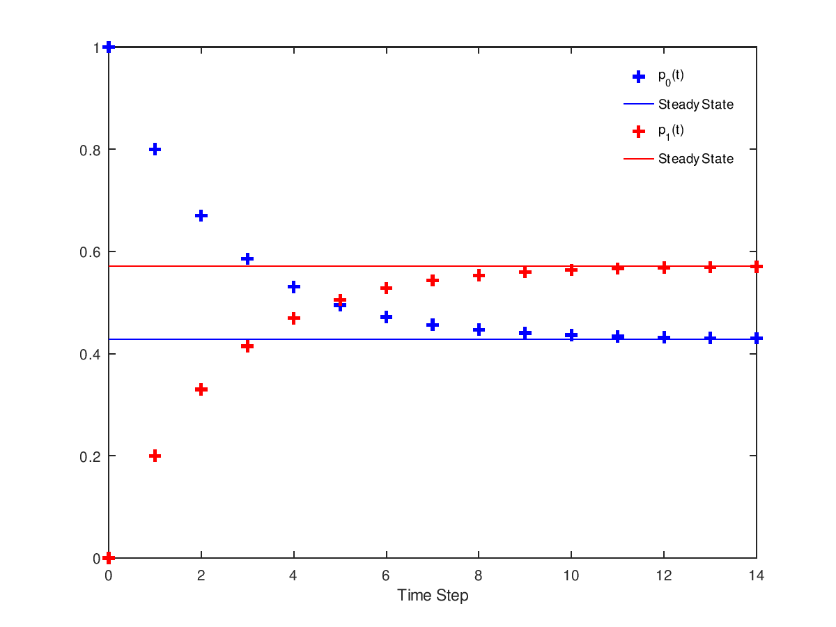
Demonstration 2

The following code

 a = 0.2;
 b = 0.15;
 P = [ 1-a a; b 1-b];
 T = 0:14;
 pp = zeros(2,length(T));
 for i=1:length(T)
   pp(:,i) = dtmc(P,T(i),[1 0]);
 endfor
 ss = dtmc(P); # compute steady state probabilities
 plot( T, pp(1,:), "b+;p_0(t);", "linewidth", 2, ...
       T, ss(1)*ones(size(T)), "b;Steady State;", ...
       T, pp(2,:), "r+;p_1(t);", "linewidth", 2, ...
       T, ss(2)*ones(size(T)), "r;Steady State;" );
 xlabel("Time Step");
 legend("boxoff");

Produces the following figure

Columns 1 through 7:

   0.083333   0.125000   0.083333   0.125000   0.166667   0.125000   0.083333

 Columns 8 and 9:

   0.125000   0.083333

Figure 1

Package: queueing