Function Reference: qncmaba

Function File: [Xl, Xu, Rl, Ru] = qncmaba (N, D)

Function File: [Xl, Xu, Rl, Ru] = qncmaba (N, S, V)

Function File: [Xl, Xu, Rl, Ru] = qncmaba (N, S, V, m)

Function File: [Xl, Xu, Rl, Ru] = qncmaba (N, S, V, m, Z)

Compute Asymptotic Bounds for closed, multiclass networks with K service centers and C customer classes. Single-server and infinite-server nodes are supported. Multiple-server nodes and general load-dependent servers are not supported.

INPUTS

N(c): number of class c requests in the system (vector of length C, N(c) ≥ 0).
D(c, k): class c service demand at center k (C \times K matrix, D(c,k) ≥ 0).
S(c, k): mean service time of class c requests at center k (C \times K matrix, S(c,k) ≥ 0).
V(c,k): average number of visits of class c requests to center k (C \times K matrix, V(c,k) ≥ 0).
m(k): number of servers at center k (if m is a scalar, all centers have that number of servers). If m(k) < 1, center k is a delay center (IS); if m(k) = 1, center k is a M/M/1-FCFS server. This function does not support multiple-server nodes. Default is 1.
Z(c): class c external delay (vector of length C, Z(c) ≥ 0). Default is 0.

OUTPUTS

Xl(c)
Xu(c): Lower and upper bounds for class c throughput.
Rl(c)
Ru(c): Lower and upper bounds for class c response time.

REFERENCES

Edward D. Lazowska, John Zahorjan, G. Scott Graham, and Kenneth C. Sevcik, Quantitative System Performance: Computer System Analysis Using Queueing Network Models, Prentice Hall, 1984. http://www.cs.washington.edu/homes/lazowska/qsp/. In particular, see section 5.2 ("Asymptotic Bounds").

See also: qncsaba.

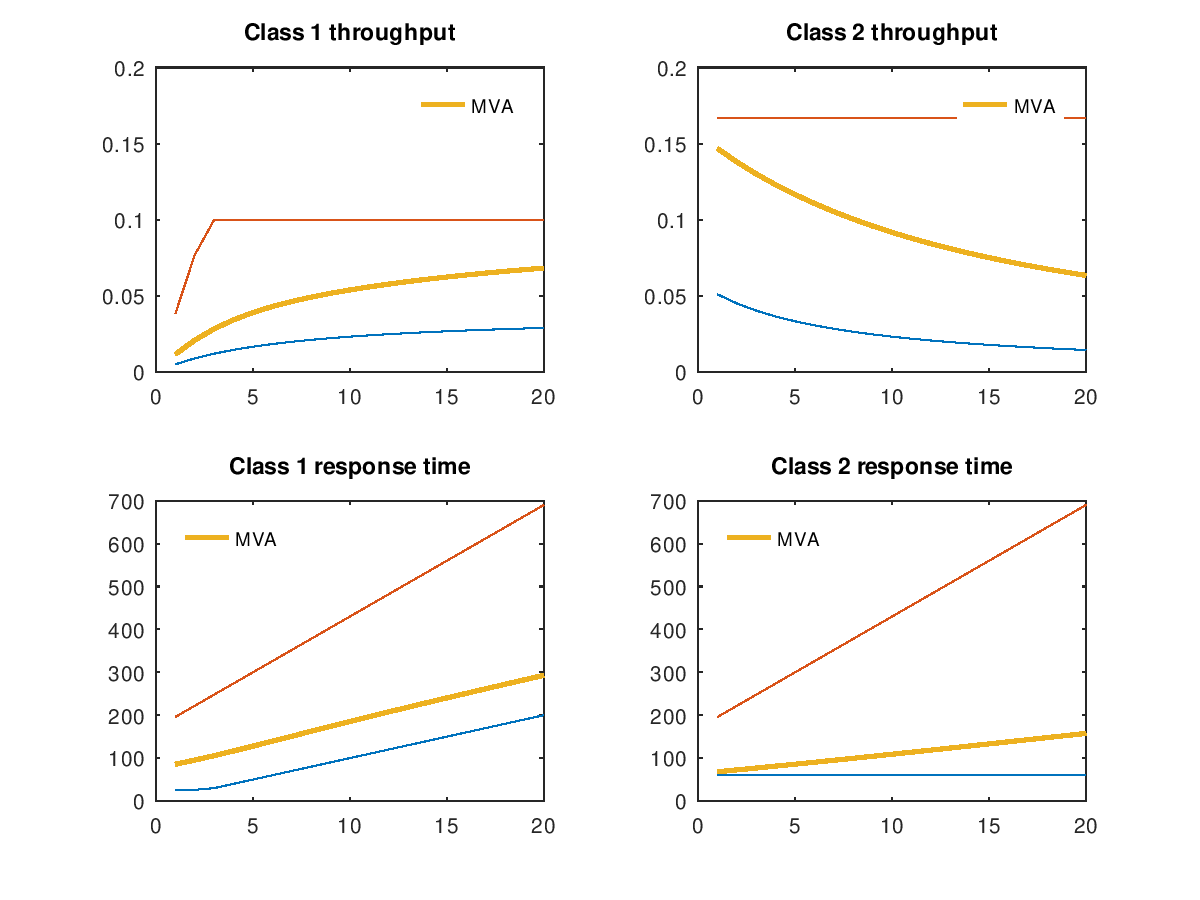
Demonstration 1

The following code

 S = [10 7 5 4; ...
      5  2 4 6];
 NN=20;
 Xl = Xu = Rl = Ru = Xmva = Rmva = zeros(NN,2);
 for n=1:NN
   N=[n,10];
   [a b c d] = qncmaba(N,S);
   Xl(n,:) = a; Xu(n,:) = b; Rl(n,:) = c; Ru(n,:) = d;
   [U R Q X] = qncmmva(N,S,ones(size(S)));
   Xmva(n,:) = X(:,1)'; Rmva(n,:) = sum(R,2)';
 endfor
 subplot(2,2,1);
 plot(1:NN,Xl(:,1), 1:NN,Xu(:,1), 1:NN,Xmva(:,1), ";MVA;", "linewidth", 2);
 ylim([0, 0.2]);
 title("Class 1 throughput"); legend("boxoff");
 subplot(2,2,2);
 plot(1:NN,Xl(:,2), 1:NN,Xu(:,2), 1:NN,Xmva(:,2), ";MVA;", "linewidth", 2);
 ylim([0, 0.2]);
 title("Class 2 throughput"); legend("boxoff");
 subplot(2,2,3);
 plot(1:NN,Rl(:,1), 1:NN,Ru(:,1), 1:NN,Rmva(:,1), ";MVA;", "linewidth", 2);
 ylim([0, 700]);
 title("Class 1 response time"); legend("location", "northwest"); legend("boxoff");
 subplot(2,2,4);
 plot(1:NN,Rl(:,2), 1:NN,Ru(:,2), 1:NN,Rmva(:,2), ";MVA;", "linewidth", 2);
 ylim([0, 700]);
 title("Class 2 response time"); legend("location", "northwest"); legend("boxoff");

Produces the following figure

Figure 1

Package: queueing