Function Reference: qncmbsb

Function File: [Xl, Xu, Rl, Ru] = qncmbsb (N, D)

Function File: [Xl, Xu, Rl, Ru] = qncmbsb (N, S, V)

Compute Balanced System Bounds for closed, multiclass networks with K service centers and C customer classes. Only single-server nodes are supported.

INPUTS

N(c): number of class c requests in the system (vector of length C).
D(c, k): class c service demand at center k (C \times K matrix, D(c,k) ≥ 0).
S(c, k): mean service time of class c requests at center k (C \times K matrix, S(c,k) ≥ 0).
V(c,k): average number of visits of class c requests to center k (C \times K matrix, V(c,k) ≥ 0).

OUTPUTS

Xl(c)
Xu(c): Lower and upper class c throughput bounds (vector of length C).
Rl(c)
Ru(c): Lower and upper class c response time bounds (vector of length C).

See also: qncsbsb.

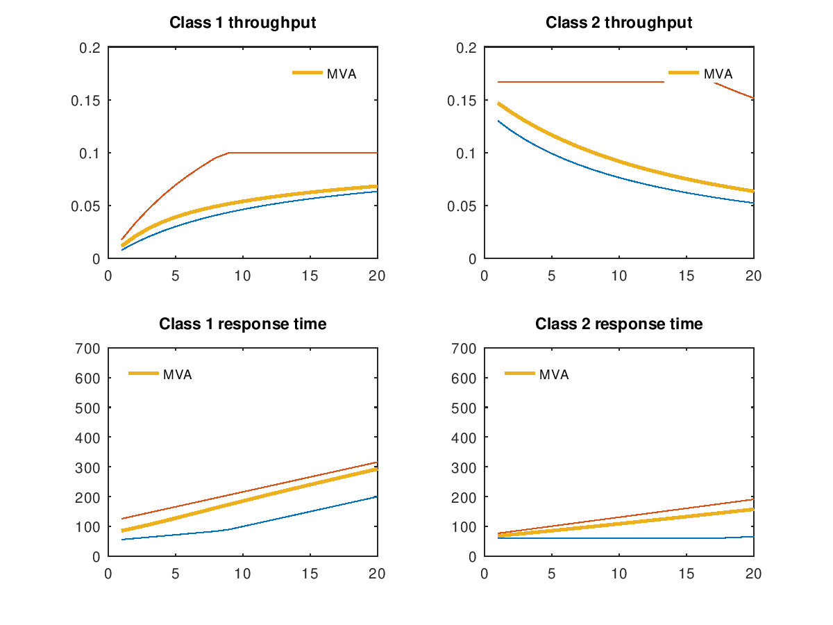
Demonstration 1

The following code

 S = [10 7 5 4; ...
      5  2 4 6];
 NN=20;
 Xl = Xu = Rl = Ru = Xmva = Rmva = zeros(NN,2);
 for n=1:NN
   N=[n,10];
   [a b c d] = qncmbsb(N,S);
   Xl(n,:) = a; Xu(n,:) = b; Rl(n,:) = c; Ru(n,:) = d;
   [U R Q X] = qncmmva(N,S,ones(size(S)));
   Xmva(n,:) = X(:,1)'; Rmva(n,:) = sum(R,2)';
 endfor
 subplot(2,2,1);
 plot(1:NN,Xl(:,1), 1:NN,Xu(:,1), 1:NN,Xmva(:,1),";MVA;", "linewidth", 2);
 ylim([0, 0.2]);
 title("Class 1 throughput"); legend("boxoff");
 subplot(2,2,2);
 plot(1:NN,Xl(:,2), 1:NN,Xu(:,2), 1:NN,Xmva(:,2),";MVA;", "linewidth", 2);
 ylim([0, 0.2]);
 title("Class 2 throughput"); legend("boxoff");
 subplot(2,2,3);
 plot(1:NN,Rl(:,1), 1:NN,Ru(:,1), 1:NN,Rmva(:,1),";MVA;", "linewidth", 2);
 ylim([0, 700]);
 title("Class 1 response time"); legend("location", "northwest"); legend("boxoff");
 subplot(2,2,4);
 plot(1:NN,Rl(:,2), 1:NN,Ru(:,2), 1:NN,Rmva(:,2),";MVA;", "linewidth", 2);
 ylim([0, 700]);
 title("Class 2 response time"); legend("location", "northwest"); legend("boxoff");

Produces the following figure

Figure 1

Package: queueing