- Function File:
[b, a] =butter(n, wc)¶ - Function File:
[b, a] =butter(n, wc, filter_type)¶ - Function File:
[z, p, g] =butter(…)¶ - Function File:
[a, b, c, d] =butter(…)¶ - Function File:
[…] =butter(…, "s")¶ Generate a Butterworth filter. Default is a discrete space (Z) filter.
The cutoff frequency, wc should be specified in radians for analog filters. For digital filters, it must be a value between zero and one. For bandpass filters, wc is a two-element vector with
w(1) < w(2).The filter type must be one of
"low","high","bandpass", or"stop". The default is"low"if wc is a scalar and"bandpass"if wc is a two-element vector.If the final input argument is
"s"design an analog Laplace space filter.Low pass filter with cutoff
pi*Wcradians:[b, a] = butter (n, Wc)
High pass filter with cutoff
pi*Wcradians:[b, a] = butter (n, Wc, "high")
Band pass filter with edges
pi*Wlandpi*Whradians:[b, a] = butter (n, [Wl, Wh])
Band reject filter with edges
pi*Wlandpi*Whradians:[b, a] = butter (n, [Wl, Wh], "stop")
Return filter as zero-pole-gain rather than coefficients of the numerator and denominator polynomials:
[z, p, g] = butter (...)
Return a Laplace space filter, Wc can be larger than 1:
[...] = butter (..., "s")
Return state-space matrices:
[a, b, c, d] = butter (...)
References:
Proakis & Manolakis (1992). Digital Signal Processing. New York: Macmillan Publishing Company.
Demonstration 1
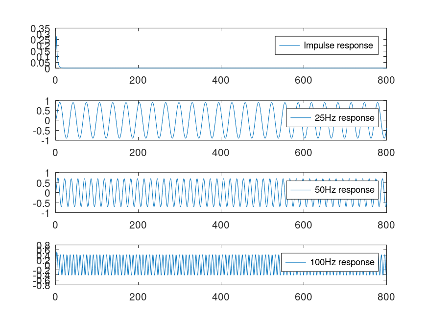
The following code
 sf = 800; sf2 = sf/2;
 data=[[1;zeros(sf-1,1)],sinetone(25,sf,1,1),sinetone(50,sf,1,1),sinetone(100,sf,1,1)];
 [b,a]=butter ( 1, 50 / sf2 );
 filtered = filter(b,a,data);

 clf
 subplot ( columns ( filtered ), 1, 1)
 plot(filtered(:,1),";Impulse response;")
 subplot ( columns ( filtered ), 1, 2 )
 plot(filtered(:,2),";25Hz response;")
 subplot ( columns ( filtered ), 1, 3 )
 plot(filtered(:,3),";50Hz response;")
 subplot ( columns ( filtered ), 1, 4 )
 plot(filtered(:,4),";100Hz response;")
Produces the following figure
| Figure 1 |
|---|
 |
Package: signal