Function Reference: chirp

Function File: chirp (t) ¶

Function File: chirp (t, f0) ¶

Function File: chirp (t, f0, t1) ¶

Function File: chirp (t, f0, t1, f1) ¶

Function File: chirp (t, f0, t1, f1, shape) ¶

Function File: chirp (t, f0, t1, f1, shape, phase) ¶

Evaluate a chirp signal at time t. A chirp signal is a frequency swept cosine wave.

t: vector of times to evaluate the chirp signal
f0: frequency at time t=0 [ 0 Hz ]
t1: time t1 [ 1 sec ]
f1: frequency at time t=t1 [ 100 Hz ]
shape: shape of frequency sweep ’linear’ f(t) = (f1-f0)*(t/t1) + f0 ’quadratic’ f(t) = (f1-f0)*(t/t1)^2 + f0 ’logarithmic’ f(t) = (f1/f0)^(t/t1) * f0
phase: phase shift at t=0

For example:

specgram (chirp ([0:0.001:5]));  # default linear chirp of 0-100Hz in 1 sec
specgram (chirp ([-2:0.001:15], 400, 10, 100, "quadratic"));
soundsc (chirp ([0:1/8000:5], 200, 2, 500, "logarithmic"), 8000);

If you want a different sweep shape f(t), use the following:

y = cos (2 * pi * integral (f(t)) + phase);

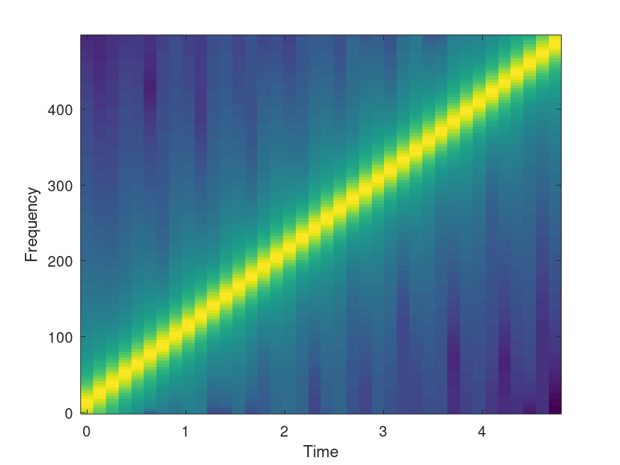
Demonstration 1

The following code

 t = 0:0.001:5;
 y = chirp (t);
 specgram (y, 256, 1000);
 %------------------------------------------------------------
 % Shows linear sweep of 100 Hz/sec starting at zero for 5 sec
 % since the sample rate is 1000 Hz, this should be a diagonal
 % from bottom left to top right.

Produces the following figure

Figure 1

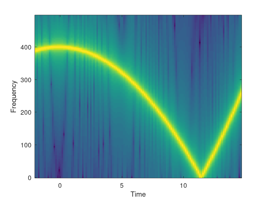
Demonstration 2

The following code

 t = -2:0.001:15;
 y = chirp (t, 400, 10, 100, "quadratic");
 [S, f, t] = specgram (y, 256, 1000);
 t = t - 2;
 imagesc(t, f, 20 * log10 (abs (S)));
 set (gca (), "ydir", "normal");
 xlabel ("Time");
 ylabel ("Frequency");
 %------------------------------------------------------------
 % Shows a quadratic chirp of 400 Hz at t=0 and 100 Hz at t=10
 % Time goes from -2 to 15 seconds.

Produces the following figure

Figure 1

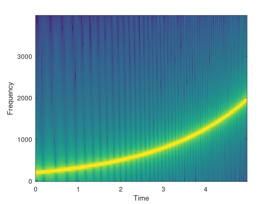
Demonstration 3

The following code

 t = 0:1/8000:5;
 y = chirp (t, 200, 2, 500, "logarithmic");
 specgram (y, 256, 8000);
 %-------------------------------------------------------------
 % Shows a logarithmic chirp of 200 Hz at t=0 and 500 Hz at t=2
 % Time goes from 0 to 5 seconds at 8000 Hz.

Produces the following figure

Figure 1

Package: signal