- Function File:
y =decimate(x, q)¶ - Function File:
y =decimate(x, q, n)¶ - Function File:
y =decimate(…, "fir")¶ -
Downsample the signal x by a reduction factor of q. A lowpass antialiasing filter is applied to the signal prior to reducing the input sequence. By default, an order n Chebyshev type I filter is used. If n is not specified, the default is 8.
If the optional argument
"fir"is given, an order n FIR filter is used, with a default order of 30 if n is not given.Note that q must be an integer for this rate change method.
Example:
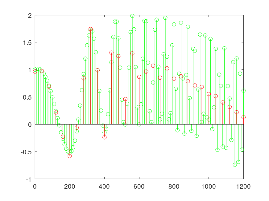
## Generate a signal that starts away from zero, is slowly varying
## at the start and quickly varying at the end, decimate and plot.
## Since it starts away from zero, you will see the boundary
## effects of the antialiasing filter clearly.  Next you will see
## how it follows the curve nicely in the slowly varying early
## part of the signal, but averages the curve in the quickly
## varying late part of the signal.
t = 0:0.01:2;
x = chirp (t, 2, .5, 10, "quadratic") + sin (2*pi*t*0.4);
y = decimate (x, 4);
stem (t(1:121) * 1000, x(1:121), "-g;Original;"); hold on; # original
stem (t(1:4:121) * 1000, y(1:31), "-r;Decimated;"); hold off; # decimated
Demonstration 1
The following code
 t=0:0.01:2; x=chirp(t,2,.5,10,'quadratic')+sin(2*pi*t*0.4);
 y = decimate(x,4);   # factor of 4 decimation
 stem(t(1:121)*1000,x(1:121),"-g;Original;"); hold on; # plot original
 stem(t(1:4:121)*1000,y(1:31),"-r;Decimated;"); hold off; # decimated
 %------------------------------------------------------------------
 % The signal to decimate starts away from zero, is slowly varying
 % at the start and quickly varying at the end, decimate and plot.
 % Since it starts away from zero, you will see the boundary
 % effects of the antialiasing filter clearly.  You will also see
 % how it follows the curve nicely in the slowly varying early
 % part of the signal, but averages the curve in the quickly
 % varying late part of the signal.
Produces the following figure
| Figure 1 |
|---|
 |
Package: signal