- Function File:
[b, a] =ellip(n, rp, rs, wp)¶ - Function File:
[b, a] =ellip(n, rp, rs, wp, "high")¶ - Function File:
[b, a] =ellip(n, rp, rs, [wl, wh])¶ - Function File:
[b, a] =ellip(n, rp, rs, [wl, wh], "stop")¶ - Function File:
[z, p, g] =ellip(…)¶ - Function File:
[a, b, c, d] =ellip(…)¶ - Function File:
[…] =ellip(…, "s")¶ -
Generate an elliptic or Cauer filter with rp dB of passband ripple and rs dB of stopband attenuation.
[b,a] = ellip(n, Rp, Rs, Wp) low pass filter with order n, cutoff pi*Wp radians, Rp decibels of ripple in the passband and a stopband Rs decibels down.
[b,a] = ellip(n, Rp, Rs, Wp, ’high’) high pass filter with cutoff pi*Wp...
[b,a] = ellip(n, Rp, Rs, [Wl, Wh]) band pass filter with band pass edges pi*Wl and pi*Wh ...
[b,a] = ellip(n, Rp, Rs, [Wl, Wh], ’stop’) band reject filter with edges pi*Wl and pi*Wh, ...
[z,p,g] = ellip(...) return filter as zero-pole-gain.
[...] = ellip(...,’s’) return a Laplace space filter, W can be larger than 1.
[a,b,c,d] = ellip(...) return state-space matrices
References:
- Oppenheim, Alan V., Discrete Time Signal Processing, Hardcover, 1999. - Parente Ribeiro, E., Notas de aula da disciplina TE498 - Processamento Digital de Sinais, UFPR, 2001/2002.
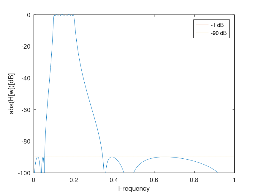
Demonstration 1
The following code
 [n, Ws] = ellipord ([.1 .2], [.01 .4], 1, 90);
 [b, a] = ellip (5, 1, 90, [.1 .2]);
 [h, w] = freqz (b, a);

 plot (w./pi, 20*log10 (abs (h)), ";;")
 xlabel ("Frequency");
 ylabel ("abs(H[w])[dB]");
 axis ([0, 1, -100, 0]);

 hold ("on");
 x=ones (1, length (h));
 plot (w./pi, x.*-1, ";-1 dB;")
 plot (w./pi, x.*-90, ";-90 dB;")
 hold ("off");
Produces the following figure
| Figure 1 |
|---|
 |
Package: signal