- Function File:
b =fir2(n, f, m)¶ - Function File:
b =fir2(n, f, m, grid_n)¶ - Function File:
b =fir2(n, f, m, grid_n, ramp_n)¶ - Function File:
b =fir2(n, f, m, grid_n, ramp_n, window)¶ -
Produce an order n FIR filter with arbitrary frequency response m over frequency bands f, returning the n+1 filter coefficients in b. The vector f specifies the frequency band edges of the filter response and m specifies the magnitude response at each frequency.
The vector f must be nondecreasing over the range [0,1], and the first and last elements must be 0 and 1, respectively. A discontinuous jump in the frequency response can be specified by duplicating a band edge in f with different values in m.
The resolution over which the frequency response is evaluated can be controlled with the grid_n argument. The default is 512 or the next larger power of 2 greater than the filter length.
The band transition width for discontinuities can be controlled with the ramp_n argument. The default is grid_n/25. Larger values will result in wider band transitions but better stopband rejection.
An optional shaping window can be given as a vector with length n+1. If not specified, a Hamming window of length n+1 is used.
To apply the filter, use the return vector b with the
filterfunction, for exampley = filter (b, 1, x).Example:
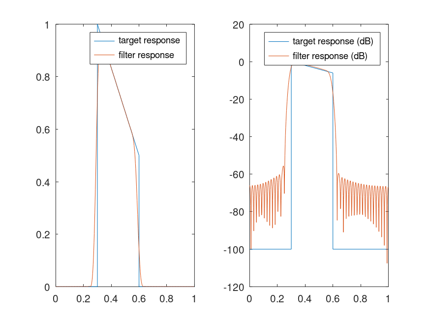
f = [0, 0.3, 0.3, 0.6, 0.6, 1]; m = [0, 0, 1, 1/2, 0, 0];
[h, w] = freqz (fir2 (100, f, m));
plot (f, m, ";target response;", w/pi, abs (h), ";filter response;");
See also: filter, fir1.
Demonstration 1
The following code
 f=[0, 0.3, 0.3, 0.6, 0.6, 1]; m=[0, 0, 1, 1/2, 0, 0];
 [h, w] = freqz(fir2(100,f,m));
 subplot(121);
 plot(f,m,';target response;',w/pi,abs(h),';filter response;');
 subplot(122);
 plot(f,20*log10(m+1e-5),';target response (dB);',...
      w/pi,20*log10(abs(h)),';filter response (dB);');
Produces the following figure
| Figure 1 |
|---|
 |
Demonstration 2
The following code
 f=[0, 0.3, 0.3, 0.6, 0.6, 1]; m=[0, 0, 1, 1/2, 0, 0];
 plot(f,20*log10(m+1e-5),';target response;');
 hold on;
 [h, w] = freqz(fir2(50,f,m,512,0));
 plot(w/pi,20*log10(abs(h)),';filter response (ramp=0);');
 [h, w] = freqz(fir2(50,f,m,512,25.6));
 plot(w/pi,20*log10(abs(h)),';filter response (ramp=pi/20 rad);');
 [h, w] = freqz(fir2(50,f,m,512,51.2));
 plot(w/pi,20*log10(abs(h)),';filter response (ramp=pi/10 rad);');
 hold off;
Produces the following figure
| Figure 1 |
|---|
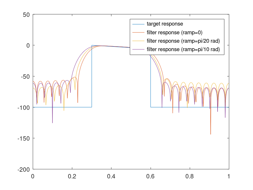 |
Demonstration 3
The following code
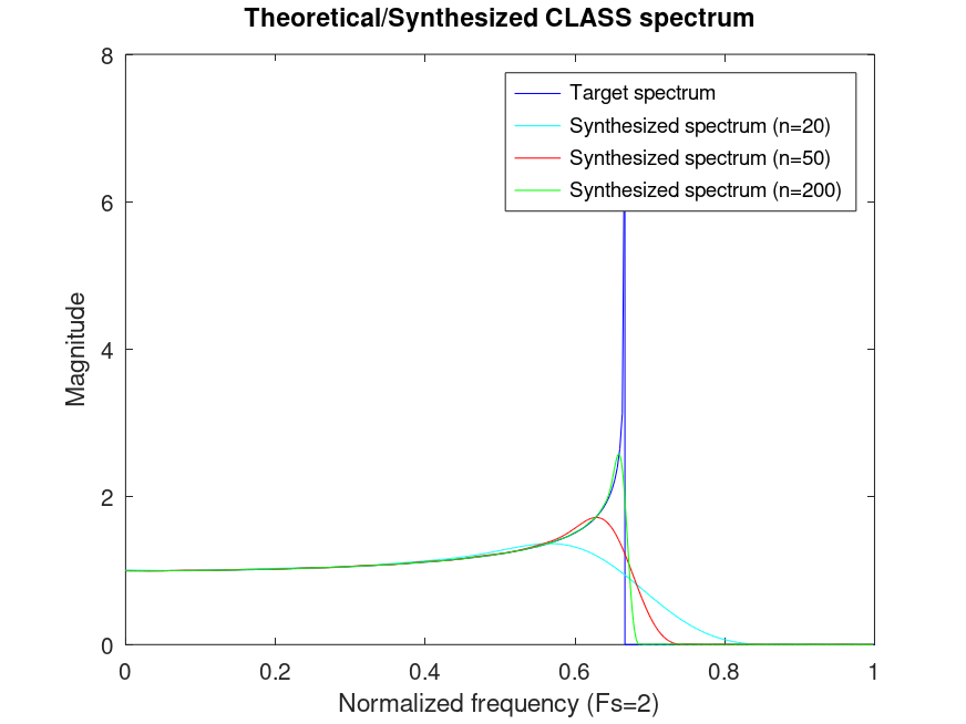
 % Classical Jakes spectrum
 % X represents the normalized frequency from 0
 % to the maximum Doppler frequency
 asymptote = 2/3;
 X = linspace(0,asymptote-0.0001,200);
 Y = (1 - (X./asymptote).^2).^(-1/4);

 % The target frequency response is 0 after the asymptote
 X = [X, asymptote, 1];
 Y = [Y, 0, 0];

 plot(X,Y,'b;Target spectrum;');
 hold on;
 [H,F]=freqz(fir2(20, X, Y));
 plot(F/pi,abs(H),'c;Synthesized spectrum (n=20);');
 [H,F]=freqz(fir2(50, X, Y));
 plot(F/pi,abs(H),'r;Synthesized spectrum (n=50);');
 [H,F]=freqz(fir2(200, X, Y));
 plot(F/pi,abs(H),'g;Synthesized spectrum (n=200);');
 hold off;
 title('Theoretical/Synthesized CLASS spectrum');
 xlabel('Normalized frequency (Fs=2)');
 ylabel('Magnitude');
Produces the following figure
| Figure 1 |
|---|
 |
Package: signal