Function Reference: firpm

Loadable Function: b = firpm (n, f, a) ¶

Loadable Function: b = firpm (n, f, @respFn) ¶

Loadable Function: b = firpm (n, f, {@respFn, …}) ¶

Loadable Function: b = firpm (…, w) ¶

Loadable Function: b = firpm (…, class) ¶

Loadable Function: b = firpm (…, {accuracy, …}) ¶

Loadable Function: [b, minimax] = firpm (…) ¶

Loadable Function: [b, minimax, res] = firpm (…) ¶

Designs a linear-phase FIR filter according to given specifications and the ‘minimax’ criterion. The method (per McClellan et al.¹) uses successive approximation to minimize the maximum weighted error between the desired and actual frequency response of the filter. Such filters are variably described as being ‘minimax’, ‘equiripple’, or ‘optimal (in the Chebyshev sense)’.

Arguments

…

Where shown as the first argument to firpm, indicates that any previously-indicated list of arguments may substitute for the ellipsis.

n

A positive integer giving the filter order.

f

A vector of real-numbers, increasing in the range [0,1], giving the frequencies of the left and right edges of each band for which a specific amplitude response is desired: [l1 r1 l2 r2 …]. 1 represents the Nyquist-frequency. Transition-bands are defined implicitly as the regions between or outside the given bands.

a

A vector of real-numbers giving the desired amplitude response. An amplitude value is given either for each band edge: [a(l1) a(r1) a(l2) a(r2) …], or for each band: [a1 a2 …]. In the former case, in-band amplitude is determined by linear interpolation between the given band-edge values. 1 represents unity-gain, 0 represents infinite attenuation, and −1 represents a phase change of pi radians.

Note that amplitude response is necessarily zero at f=0 for type III and IV filters, and at f=1 for type II and III filters.

@respFn

A handle to a ‘response function’ that supplies the desired amplitude response and error-weighting. This, unlike a above, allows the response to be arbitrary (subject to the note above). firpm invokes the response function according to the following syntax:

ag = respFn (n,f,g,w, …)
[ag wg] = respFn (n,f,g,w, …)
symmetry = respFn ("defaults", {n,f,g,w, …})

where:

n and f are as given to firpm.
w is as given to firpm, or ones if not given.
ag and wg are the desired amplitude and weighting functions evaluated at each frequency in vector g (which are frequencies within the non-transition bands of f). Returning ag alone gives uniform weighting.
symmetry is either "even" or "odd"; this provides an alternative to using the class values "symmetric" and "antisymmetric".
Per the ellipses shown here and above, when @respFn is given contained in a cell-array, any additionally contained values are appended to the respFn invocation argument-list.

w

When used in conjunction with a, w is a vector of positive real-numbers giving error-weightings to be applied at each given band-edge [w(l1) w(r1) w(l2) w(r2) …], or for each band [w1 w2 …]. In the former case, in-band weighting is determined by linear interpolation between the given band-edge values. A higher relative error weighting yields a lower relative error.

When used in conjunction with @respFn, w is a vector (constrained as above) that is passed through to respFn.

class

A string, which may be abbreviated, giving the filter-class:

"symmetric" (the default) for type I or II filters,
"antisymmetric" (or "hilbert") for standard type III or IV filters,
"differentiator" for type III or IV filters with inverted phase and with error-weighting (further to w) of 2/f applied in the pass-band(s).

accuracy, …

Up to three properties contained within a cell-array: accuracy, persistence, robustness, that respectively control how close the computed filter will be to the ideal minimax solution, the number of computation iterations over which the required accuracy will be sought, and the precision of certain internal processing. Each can each be set to a small positive number (typically ≤3), to increase the relevant item; this may increase computation time, but the need to do so should be rare. A value of 0 can be used to leave an item unchanged.

Alternatively, setting accuracy ≥16 emulates MATLAB’s lgrid argument.

Results

If a problem occurs during the computation, a diagnostic message will normally be displayed. If this happens, adjusting accuracy, persistence, or robustness may provide the solution. Some filters however, may not be realizable due to machine-precision limitations. If a filter can be computed, returned values are as follows:

b

A length N+1 row-vector containing the computed filter coefficients.

minimax

The absolute value of the minimized, maximum weighted error, or this number negated if the required accuracy could not be achieved.

res

A structure of data relating to the filter computation and a partial response-analysis of the resultant filter; fields are vectors:

fgrid Analysis frequencies per f.

des Desired amplitude response.

wt Error weighting.

H Complex frequency response.

error Desired minus actual amplitude response.

iextr Indices of local peaks in error.

fextr Frequencies of local peaks in error.

Using res is not recommended because it can be slow to compute and, since the analysis excludes transition-bands, any ‘anomalies’² therein are not easy to discern. In general, freqz suffices to check that the response of the computed filter is satisfactory.

Examples

# Low-pass with frequencies in Hz:
Fs = 96000; Fn = Fs/2; # Sampling & Nyquist frequencies.
b = firpm (50, [0 20000 28000 48000] / Fn, [1 0]);

# Type IV high-pass:
b = firpm (31, [0 0.5 0.7 1], [0 1], "antisym");

# Inverse-sinc (arbitrary response):
b = firpm (20, [0 0.5 0.9 1], @(n,f,g) ...
   deal ((g<=f(2))./sinc (g), (g>=f(3))*9+1));

# Band-pass with filter-response check:
freqz (firpm (40, [0 3 4 6 8 10]/10, [0 1 0]))

Further examples can be found in the firpm and firpmord demonstration scripts.

Compatibility

Given invalid filter specifications, Octave emits an error and does not produce a filter; MATLAB in such circumstances may still produce filter coefficients.

Unlike with MATLAB, with Octave minimax can be negative; for compatibility, take the absolute value.

See also: firpmord.

Demonstration 1

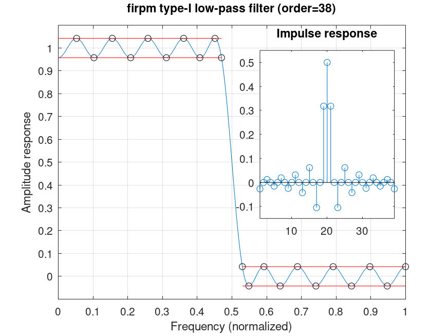
The following code


 N=38; F=[0 .47 .53 1]; A=[1 1 0 0]; W=[1 1]; ant=0;
 [b m r] = firpm (N, F, A, W, 'sa'(1+ant));

 mul=[1 i](1+ant);
 clf; [h f] = freqz (b); plot (f/pi, real (mul*h.*exp (i*f*N/2)),
     f=F(1:2),(a=A(1:2))-(M=m/W(1)),'r', f, a+M,'r',
     f=F(3:4),(a=A(3:4))-(M=m/W(2)),'r', f, a+M,'r',
     r.fextr, real ((mul*r.H.*exp (i*r.fgrid*pi*N/2))(r.iextr)),'ko')
 grid on; axis ([0 1 -.1 1.1]); set (gca, 'xtick', [0:.1:1], 'ytick', [0:.1:1])
 title (sprintf ('firpm type-I low-pass filter (order=%i)', length (b) - 1));
 ylabel ('Amplitude response'); xlabel ('Frequency (normalized)')
 axes ('position', [.58 .35 .3 .5])
 stem (b); grid off
 title ('Impulse response')
 axis ([1 length(b) -.15 .55])
 %--------------------------------------------------
 % Figure shows transfer and impulse-response of
 % half-band filter design.

Produces the following figure

Figure 1

Demonstration 2

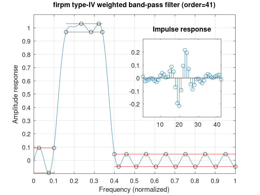
The following code


 N=41; F=[0 .1 .16 .34 .4 1]; A=[0 0 1 1 0 0]; W=[1 3 2]; ant=1;
 [b m r] = firpm (N, F, A, W, 'sa'(1+ant));

 mul=[1 i](1+ant);
 clf; [h f] = freqz (b); plot (f/pi, real (mul*h.*exp (i*f*N/2)),
     f=F(1:2),(a=A(1:2))-(M=m/W(1)),'r', f, a+M,'r',
     f=F(3:4),(a=A(3:4))-(M=m/W(2)),'r', f, a+M,'r',
     f=F(5:6),(a=A(5:6))-(M=m/W(3)),'r', f, a+M,'r',
     r.fextr, real ((mul*r.H.*exp (i*r.fgrid*pi*N/2))(r.iextr)),'ko')
 grid on; axis ([0 1 -.1 1.1]); set (gca, 'xtick', [0:.1:1], 'ytick', [0:.1:1])
 title (sprintf ('firpm type-IV weighted band-pass filter (order=%i)', length (b) - 1));
 ylabel ('Amplitude response'); xlabel ('Frequency (normalized)')
 axes ('position', [.55 .4 .3 .4])
 stem (b); grid off
 title ('Impulse response')
 axis ([1 length(b) -.3 .3])
 %--------------------------------------------------
 % Figure shows transfer and impulse-response of
 % band-pass filter design.

Produces the following figure

Figure 1

Demonstration 3

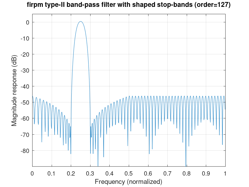
The following code


 curve = @(a,b,y,z,x) z*(b-a)./((x-a)*z/y+b-x);
 respFn = @(n,f,g,w,curve) deal (g>=f(3) & g<=f(4), ...
   (g<=f(2)).*curve (f(2),f(1),w(1),w(3),g) + ...
   (g>=f(3) & g<=f(4))*w(2) + ...
   (g>=f(5) & g<=f(6)).*curve (f(5),f(6),w(1),w(3),g) + ...
   (g>f(7))*w(4)); % NB contiguous bands so > not >=.
 b=firpm (127, [0 .2 .24 .26 .3 .5 .5 1], {respFn, curve}, [10 1 100 10]);

 clf; [h f]=freqz (b); plot (f/pi, 20*log10 (abs (h)))
 grid on; axis ([0 1 -90 5]); set (gca, 'xtick', [0:.1:1], 'ytick', [-80:10:0])
 title (sprintf ('firpm type-II band-pass filter with shaped stop-bands (order=%i)', length (b) - 1));
 ylabel ('Magnitude response (dB)'); xlabel ('Frequency (normalized)')
 %--------------------------------------------------
 % Figure shows transfer of band-pass filter design
 % with shaped error-weight in the stop-bands.

Produces the following figure

Figure 1

Demonstration 4

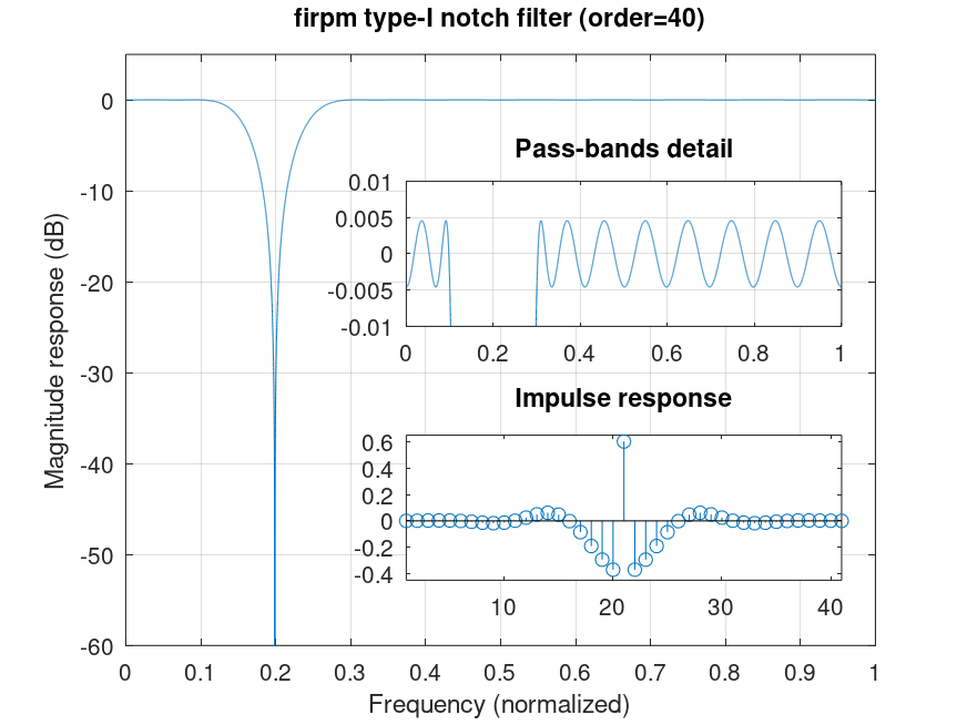
The following code


 b = firpm (40, [0 .1 .3 1], [-1 1]);

 clf; [h f] = freqz (b,1,2^14); plot (f/pi, 20*log10 (abs (h)))
 grid on; axis ([0 1 -60 5]); set (gca, 'xtick', [0:.1:1])
 title (sprintf ('firpm type-I notch filter (order=%i)', length (b) - 1));
 ylabel ('Magnitude response (dB)'); xlabel ('Frequency (normalized)')
 axes ('position', [.42 .55 .45 .2])
 plot (f/pi, 20*log10 (abs (h))); grid on
 axis ([0 1 -(e=1e-2) e])
 title ('Pass-bands detail')
 axes ('position', [.42 .2 .45 .2])
 stem (b); grid off
 title ('Impulse response')
 axis ([1 length(b) -.45 .65])
 %--------------------------------------------------
 % Figure shows transfer and impulse-response of
 % notch filter design.

Produces the following figure

Figure 1

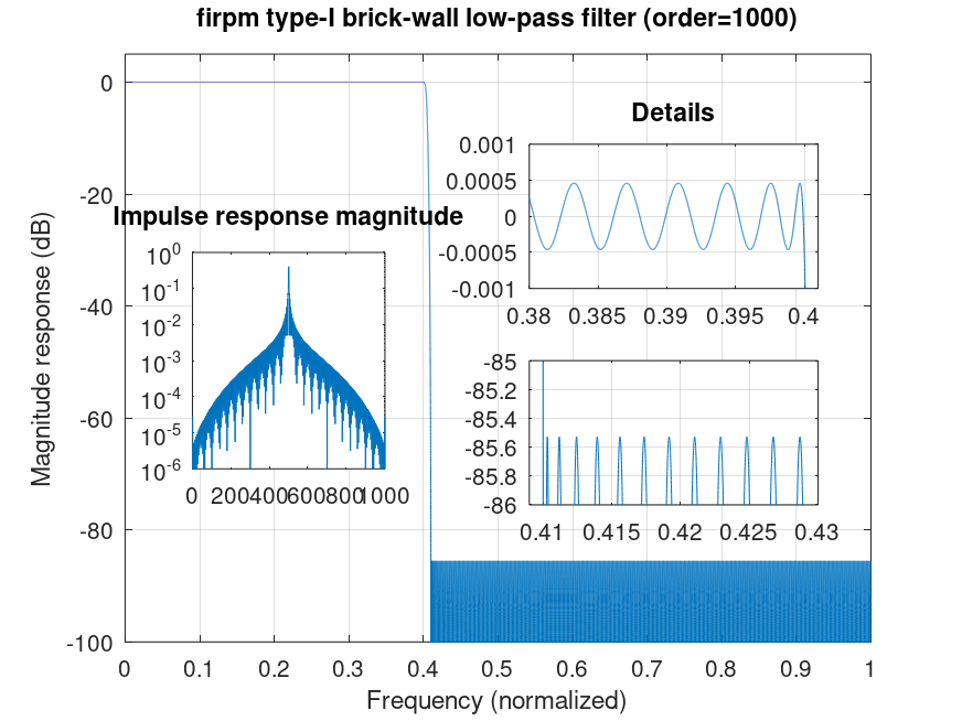
Demonstration 5

The following code


 b = firpm (1000, [0 .4 .41 1], [1 0], {1});

 clf; [h f] = freqz (b, 1, 2^17); plot (f/pi, 20*log10 (abs (h)))
 title (sprintf ('firpm type-I brick-wall low-pass filter (order=%i)', length (b) - 1));
 ylabel ('Magnitude response (dB)'); xlabel ('Frequency (normalized)')
 grid on; axis ([0 1 -100 5]); set (gca, 'xtick', [0:.1:1])
 axes ('position', [.55 .6 .3 .2])
 plot (f/pi, 20*log10 (abs (h))); grid on
 title ('Details')
 axis ([.38 .401 -(e=1e-3) e])
 axes ('position', [.55 .3 .3 .2])
 plot (f/pi, 20*log10 (abs (h))); grid on
 axis ([.409 .43 -86 -85])
 axes ('position', [.2 .35 .2 .3])
 semilogy (abs (b)); grid off
 title ('Impulse response magnitude')
 axis ([0 length(b)+1 1e-6 1])
 %--------------------------------------------------
 % Figure shows transfer and impulse-response of
 % brick-wall low-pass filter design.

Produces the following figure

Figure 1

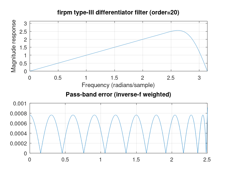
Demonstration 6

The following code


 b = firpm (20, [0 2.5]/pi, [0 2.5], 'differentiator');

 clf
 [h f] = freqz (b,1,2^12);
 subplot (2, 1, 1)
 plot (f, abs (h)); grid on
 title (sprintf ('firpm type-III differentiator filter (order=%i)', length (b) - 1));
 ylabel ('Magnitude response'); xlabel ('Frequency (radians/sample)')
 axis ([0 pi 0 pi])
 subplot (2, 1, 2)
 plot (f, abs (abs (h)./f-1)); grid on
 axis ([0 2.5 0 1e-3])
 title ('Pass-band error (inverse-f weighted)')
 %--------------------------------------------------
 % Figure shows transfer of differentiator filter design.
 % above: full-band
 % below: detail of pass-band error (inverse-f weighted)

Produces the following figure

Figure 1

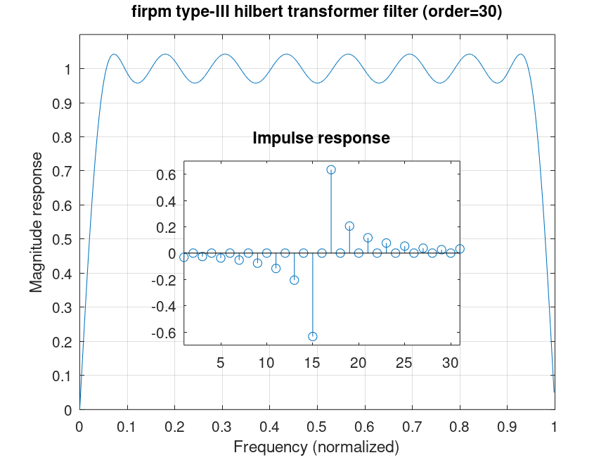
Demonstration 7

The following code


 b = firpm (30, [.05 .95], 1, 'antisymmetric');

 clf; [h f] = freqz (b); plot (f/pi, abs (h))
 grid on; axis ([0 1 0 1.1]); set (gca, 'xtick', [0:.1:1], 'ytick', [0:.1:1])
 title (sprintf ('firpm type-III hilbert transformer filter (order=%i)', length (b) - 1));
 ylabel ('Magnitude response'); xlabel ('Frequency (normalized)')
 axes ('position', [.3 .25 .45 .4])
 stem (b); grid off
 title ('Impulse response')
 axis ([1 length(b) -.7 .7])
 %--------------------------------------------------
 % Figure shows transfer and impulse-response of
 % hilbert filter design.

Produces the following figure

Figure 1

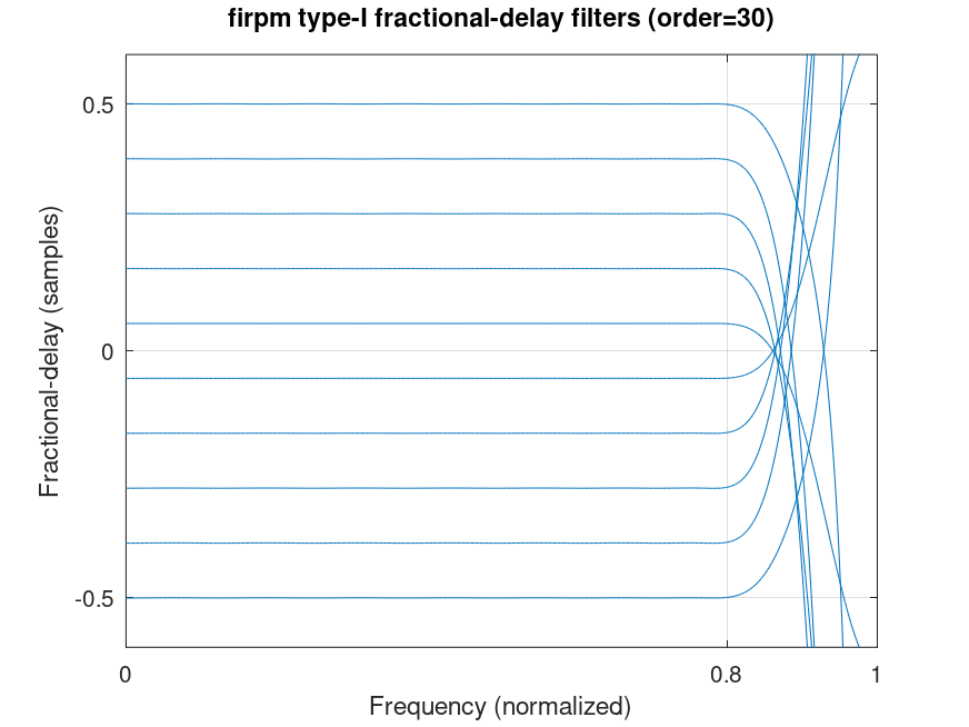
Demonstration 8

The following code

 clf; n=30; Fp=.8; for d=linspace (-.5, .5, 10)

 b = firpm (n, [0 Fp], {@(n,f,g,w,d,Fp) (g<=Fp).*cos (g*pi*d),d,Fp})...
   + firpm (n, [0 Fp], {@(n,f,g,w,d,Fp) (g<=Fp).*sin (g*pi*d),d,Fp}, 'a');

 [g f]=grpdelay (b);
 set (gca,'ColorOrderIndex',1); plot (f/pi, g-n/2); hold ('on'); end;
 hold ('off'); grid on; axis ([0 1 -.6 .6]); set (gca, 'xtick', [0 Fp 1], 'ytick', [-.5:.5:.5])
 title (sprintf ('firpm type-I fractional-delay filters (order=%i)', length (b) - 1));
 ylabel ('Fractional-delay (samples)'); xlabel ('Frequency (normalized)')
 %--------------------------------------------------
 % Figure shows delay response of (non-linear-phase)
 % filter designs with progressive fractional-delay.

Produces the following figure

Figure 1

Package: signal

`fgrid`	Analysis frequencies per `f`.
`des`	Desired amplitude response.
`wt`	Error weighting.
`H`	Complex frequency response.
`error`	Desired minus actual amplitude response.
`iextr`	Indices of local peaks in `error`.
`fextr`	Frequencies of local peaks in `error`.