- Function File:
[n, Fout, a, w] =firpmord(f, a, d)¶ - Function File:
[n, Fout, a, w] =firpmord(f, a, d, fs)¶ - Function File:
c =firpmord(f, a, d, "cell")¶ - Function File:
c =firpmord(f, a, d, fs, "cell")¶ -
Estimate the filter-order needed for
firpmto design a type-I or type-II linear-phase FIR filter according to the given specifications.Arguments 
- f
A vector of real-numbers, increasing in the range (0, fs/2), giving the frequencies of the left and right edges of each band for which a specific amplitude response is desired (omitting 0 and fs/2, which are implied): [r1 l2 r2 …]. Transition-bands are defined implicitly as the regions between the given bands.
- a
A vector of real-numbers giving the ideal amplitude response. An amplitude value is given for each band specified by f: [a1 a2 …]. 1 represents unity-gain, 0 represents infinite attenuation, and −1 represents a phase change of pi radians.
- d
A vector of positive real-numbers giving the maximum allowable linear deviation from the amplitudes given in a, thus constraining the actual amplitude response (where defined by f) to be within a +/− d. Note that, though related, d does not equate to
firpm’s w argument.- fs
-
The sampling-frequency, which defaults to 2.
Usage 
The function returns the estimated filter-order, together with the other design specification values, in one of two forms suitable for use with
firpm. By default, multiple return values are used; alternatively, by giving"cell"(or"c") as the last argument tofirpmord, the returned values are contained within a cell-array that can, if desired, be passed directly tofirpm.The following examples illustrate the use of both mechanisms, as well as aspects of
firpmordusage in general:# Low-pass; frequencies in kHz: [n f a w] = firpmord ([2.5 3], [1 0], [0.01 db2mag(-60)], 8); b = firpm (n, f, a, w);
# Band-pass:
c = firpmord ([3 4 8 9], [0 1 0], [1e-3 1e-2 1e-3], 20, "cell");
b = firpm (c{:});
# High-pass: b = firpm (firpmord ([6.4 8]/16, [0 1], [1e-4 0.01], "c"){:});In cases where elements of d follow a repeating pattern (e.g. all the elements are equal, or elements corresponding to pass-bands are equal and elements corresponding to stop-bands are equal), only as many elements as are needed to establish the pattern need be given.
For example, the following
firpmordinvocation pairs are equivalent:# Low-pass: firpmord ([0.4 0.5], [0 1], [db2mag(-72) db2mag(-72)]); firpmord ([0.4 0.5], [0 1], [db2mag(-72)]);
# Multi-band-pass:
ds = db2mag(-80); dp = 0.01;
firpmord ([1 2 3 4 5 6 7 8]/10, [0 1 0 1 0], [ds dp ds dp ds]);
firpmord ([1 2 3 4 5 6 7 8]/10, [0 1 0 1 0], [ds dp]);
Notes 
The estimation algorithm used is per Ichige et al.1 Accuracy tends to decrease as the number of bands increases. Even with two bands (i.e. high-pass or low-pass), the algorithm may under- or over-estimate. See the
firpmorddemonstrations for some examples.In order to precisely determine the minimum order needed for a particular design,
firpmordcould be used to seed an algorithm iterating invocations offirpm(as exemplified in demonstration number five).Related documentation 
See also: firpm, kaiserord.
Demonstration 1
The following code
db2mag = @(x) 10^(x/20);
fs = 8000;
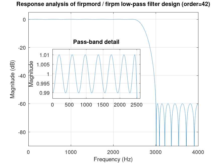
[n f a w] = firpmord ([2500 3000], [1 0], [0.01 db2mag(-60)], fs);
b = firpm (n, f, a, w);
[h f] = freqz (b, 1, 2^14); clf
plot (fs/2*f/pi, 20*log10 (abs (h))); grid on; axis ([0 fs/2 -90 5])
ylabel ("Magnitude (dB)"); xlabel ("Frequency (Hz)")
title (sprintf ("Response analysis of firpmord / firpm low-pass filter design (order=%i)", length (b) - 1))
axes ("position", [.24 .4 .4 .3])
plot (fs/2*f/pi, abs (h)); grid on; axis ([0 2600 x=.987 2-x])
ylabel ("Magnitude")
title ("Pass-band detail")
%--------------------------------------------------
% Figure shows analysis of filter designed using
% firpm with firpmord; specs. are almost met.
Produces the following figure
| Figure 1 |
|---|
 |
Demonstration 2
The following code
db2mag = @(x) 10^(x/20);
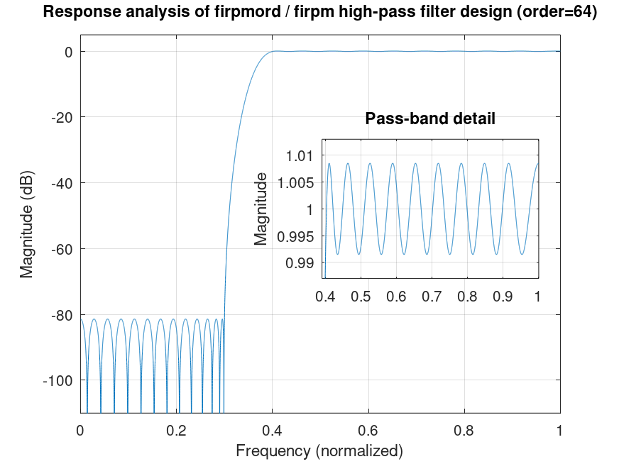
b = firpm (firpmord ([0.3 0.4], [0 1], [db2mag(-80) .01], "c"){:});
[h f] = freqz (b, 1, 2^14); clf
plot (f/pi, 20*log10 (abs (h))); grid on; axis ([0 1 -110 5])
ylabel ("Magnitude (dB)"); xlabel ("Frequency (normalized)")
title (sprintf ("Response analysis of firpmord / firpm high-pass filter design (order=%i)", length (b) - 1))
axes ("position", [.52 .4 .35 .3])
plot (f/pi, abs (h)); grid on; axis ([.39 1 x=.987 2-x])
ylabel ("Magnitude")
title ("Pass-band detail")
%--------------------------------------------------
% Figure shows analysis of filter designed using
% firpm with firpmord; specs. are exceeded.
Produces the following figure
| Figure 1 |
|---|
 |
Demonstration 3
The following code
db2mag = @(x) 10^(x/20);
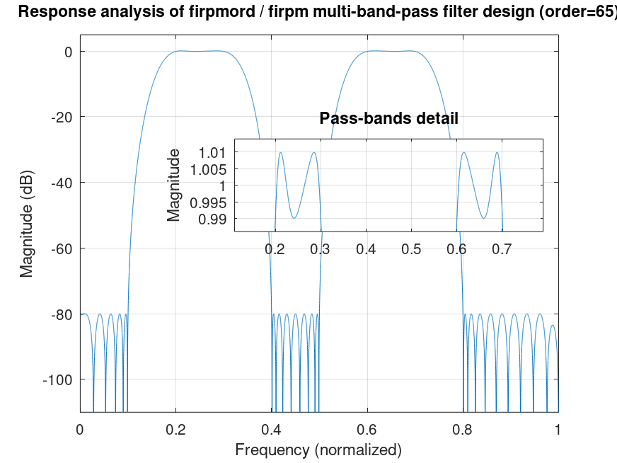
ds = db2mag (-80); dp = 0.01;
b = firpm (firpmord ([1 2 3 4 5 6 7 8]/10, [0 1 0 1 0], [ds dp], "c"){:});
[h f] = freqz (b, 1, 2^14); clf
plot (f/pi, 20*log10 (abs (h))); grid on; axis ([0 1 -110 5])
ylabel ("Magnitude (dB)"); xlabel ("Frequency (normalized)")
title ("Response analysis of firpmord / firpm multi-band-pass filter design")
title (sprintf ("Response analysis of firpmord / firpm multi-band-pass filter design (order=%i)", length (b) - 1))
axes ("position", [.38 .5 .5 .2])
plot (f/pi, abs (h)); grid on; axis ([.11 .79 x=.986 2-x])
ylabel ("Magnitude")
title ("Pass-bands detail")
%--------------------------------------------------
% Figure shows analysis of filter designed using
% firpm with firpmord; specs. are met.
Produces the following figure
| Figure 1 |
|---|
 |
Demonstration 4
The following code
db2mag = @(x) 10^(x/20);
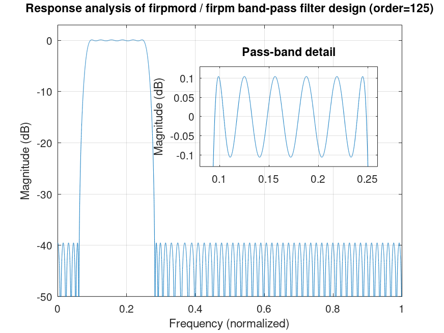
ds = db2mag (-40); dp = 1 - db2mag (-0.1);
b = firpm (firpmord ([2 3 8 9]/32, [0 1 0], [ds dp], "c"){:});
[h f] = freqz (b, 1, 2^14); clf
plot (f/pi, 20*log10 (abs (h))); grid on; axis ([0 1 -50 3])
ylabel ("Magnitude (dB)"); xlabel ("Frequency (normalized)")
title (sprintf ("Response analysis of firpmord / firpm band-pass filter design (order=%i)", length (b) - 1))
axes ("position", [.45 .5 .4 .3])
plot (f/pi, 20*log10 (abs (h))); grid on; axis ([.08 .26 x=-.13 -x])
ylabel ("Magnitude (dB)")
title ("Pass-band detail")
%--------------------------------------------------
% Figure shows analysis of filter designed using
% firpm with firpmord; specs. are not met.
Produces the following figure
| Figure 1 |
|---|
 |
Demonstration 5
The following code
% FIRPMX: F, A, D, Fs are as firpmord.
% type in {0,1,2} constrains order to be {even,odd,either} resp.
function h = firpmx (type, F, A, D, Fs = 2)
type *= !A(end); step = 2; bounds = [0 0];
while (bounds(2) - bounds(1) != step)
if all (!bounds) [n f a w] = firpmord (F, A, D, Fs);
elseif (!bounds(1)) n = min (n - step, round (n * 0.994));
elseif (!bounds(2)) n = max (n + step, round (n / 0.998));
else n = fix (mean (bounds));
endif
n += rem (n + rem (type, 2), step);
[b m] = firpm (n, f, a, w);
bounds(1 + (met = (abs(m) <= max (D)))) = n;
step -= bounds(2) - bounds(1) == type;
if (met) h = b; endif
endwhile
endfunction
db2mag = @(x) 10^(x/20);
ds = db2mag (-40); dp = 1 - db2mag (-0.1);
b = firpmx (2, [2 3 8 9]/32, [0 1 0], [ds dp]);
[h f] = freqz (b, 1, 2^14); clf
plot (f/pi, 20*log10 (abs (h))); grid on; axis ([0 1 -50 3])
ylabel ("Magnitude (dB)"); xlabel ("Frequency (normalized)")
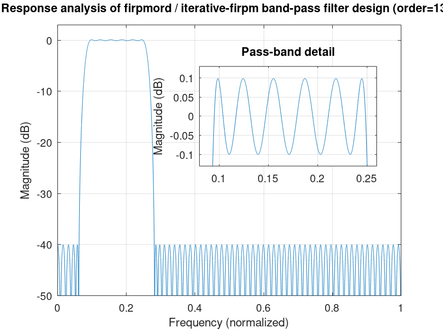
title (sprintf ("Response analysis of firpmord / iterative-firpm band-pass filter design (order=%i)", length (b) - 1))
axes ("position", [.45 .5 .4 .3])
plot (f/pi, 20*log10 (abs (h))); grid on; axis ([.08 .26 x=-.13 -x])
ylabel ("Magnitude (dB)")
title ("Pass-band detail")
%--------------------------------------------------
% Figure shows analysis of filter designed iteratively
% using firpm with firpmord, so that specs. are met.
Produces the following figure
| Figure 1 |
|---|
 |
Package: signal