- Function File:
[g, w] =grpdelay(b)¶ - Function File:
[g, w] =grpdelay(b, a)¶ - Function File:
[g, w] =grpdelay(…, n)¶ - Function File:
[g, w] =grpdelay(…, n, "whole")¶ - Function File:
[g, f] =grpdelay(…, n, Fs)¶ - Function File:
[g, f] =grpdelay(…, n, "whole", Fs)¶ - Function File:
[g, w] =grpdelay(…, w)¶ - Function File:
[g, f] =grpdelay(…, f, Fs)¶ - Function File: grpdelay
(…)¶ Compute the group delay of a filter.
[g, w] = grpdelay(b) returns the group delay g of the FIR filter with coefficients b. The response is evaluated at 512 angular frequencies between 0 and pi. w is a vector containing the 512 frequencies. The group delay is in units of samples. It can be converted to seconds by multiplying by the sampling period (or dividing by the sampling rate fs).
[g, w] = grpdelay(b,a) returns the group delay of the rational IIR filter whose numerator has coefficients b and denominator coefficients a.
[g, w] = grpdelay(b,a,n) returns the group delay evaluated at n angular frequencies. For fastest computation n should factor into a small number of small primes.
[g, w] = grpdelay(b,a,n,’whole’) evaluates the group delay at n frequencies between 0 and 2*pi.
[g, f] = grpdelay(b,a,n,Fs) evaluates the group delay at n frequencies between 0 and Fs/2.
[g, f] = grpdelay(b,a,n,’whole’,Fs) evaluates the group delay at n frequencies between 0 and Fs.
[g, w] = grpdelay(b,a,w) evaluates the group delay at frequencies w (radians per sample).
[g, f] = grpdelay(b,a,f,Fs) evaluates the group delay at frequencies f (in Hz).
grpdelay(...) plots the group delay vs. frequency.
If the denominator of the computation becomes too small, the group delay is set to zero. (The group delay approaches infinity when there are poles or zeros very close to the unit circle in the z plane.)
Theory: group delay, g(w) = -d/dw [arg{H(e^jw)}], is the rate of change of phase with respect to frequency. It can be computed as:
              d/dw H(e^-jw)
       g(w) = -------------
                H(e^-jw)
where
H(z) = B(z)/A(z) = sum(b_k z^k)/sum(a_k z^k).
By the quotient rule,
                   A(z) d/dw B(z) - B(z) d/dw A(z)
       d/dw H(z) = -------------------------------
                              A(z) A(z)
Substituting into the expression above yields:
               A dB - B dA
       g(w) =  ----------- = dB/B - dA/A
                   A B
Note that,
       d/dw B(e^-jw) = sum(k b_k e^-jwk)
       d/dw A(e^-jw) = sum(k a_k e^-jwk)
which is just the FFT of the coefficients multiplied by a ramp.
As a further optimization when nfft>>length(a), the IIR filter (b,a) is converted to the FIR filter conv(b,fliplr(conj(a))). For further details, see http://ccrma.stanford.edu/~jos/filters/Numerical_Computation_Group_Delay.html
Demonstration 1
The following code
 % 1
 %--------------------------------------------------------------
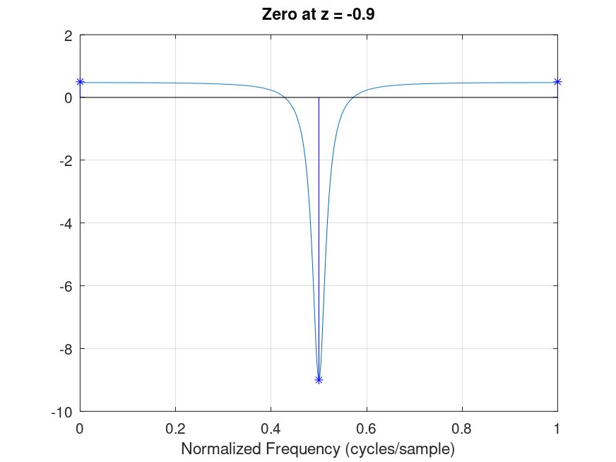
 % From Oppenheim and Schafer, a single zero of radius r=0.9 at
 % angle pi should have a group delay of about -9 at 1 and 1/2
 % at zero and 2*pi.
 %--------------------------------------------------------------
 grpdelay([1 0.9],[],512,'whole',1);
 hold on;
 xlabel('Normalized Frequency (cycles/sample)');
 stem([0, 0.5, 1],[0.5, -9, 0.5],'*b;target;');
 hold off;
 title ('Zero at z = -0.9');
Produces the following figure
| Figure 1 |
|---|
 |
Demonstration 2
The following code
 % 2
 %--------------------------------------------------------------
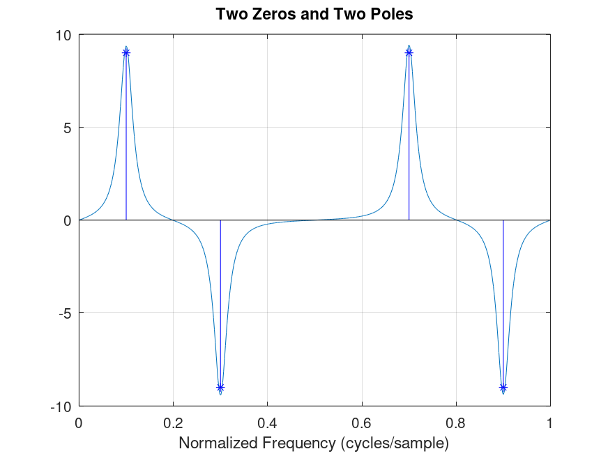
 % confirm the group delays approximately meet the targets
 % don't worry that it is not exact, as I have not entered
 % the exact targets.
 %--------------------------------------------------------------
 b = poly([1/0.9*exp(1i*pi*0.2), 0.9*exp(1i*pi*0.6)]);
 a = poly([0.9*exp(-1i*pi*0.6), 1/0.9*exp(-1i*pi*0.2)]);
 grpdelay(b,a,512,'whole',1);
 hold on;
 xlabel('Normalized Frequency (cycles/sample)');
 stem([0.1, 0.3, 0.7, 0.9], [9, -9, 9, -9],'*b;target;');
 hold off;
 title ('Two Zeros and Two Poles');
Produces the following figure
| Figure 1 |
|---|
 |
Demonstration 3
The following code
 % 3
 %--------------------------------------------------------------
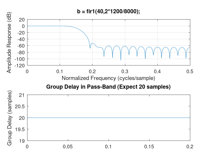
 % fir lowpass order 40 with cutoff at w=0.3 and details of
 % the transition band [.3, .5]
 %--------------------------------------------------------------
 subplot(211);
 Fs = 8000;     % sampling rate
 Fc = 0.3*Fs/2; % lowpass cut-off frequency
 nb = 40;
 b = fir1(nb,2*Fc/Fs); % matlab freq normalization: 1=Fs/2
 [H,f] = freqz(b,1,[],1);
 [gd,f] = grpdelay(b,1,[],1);
 plot(f,20*log10(abs(H)));
 title(sprintf('b = fir1(%d,2*%d/%d);',nb,Fc,Fs));
 xlabel('Normalized Frequency (cycles/sample)');
 ylabel('Amplitude Response (dB)');
 grid('on');
 subplot(212);
 del = nb/2; % should equal this
 plot(f,gd);
 title(sprintf('Group Delay in Pass-Band (Expect %d samples)',del));
 ylabel('Group Delay (samples)');
 axis([0, 0.2, del-1, del+1]);
Produces the following figure
| Figure 1 |
|---|
 |
Demonstration 4
The following code
 % 4
 %--------------------------------------------------------------
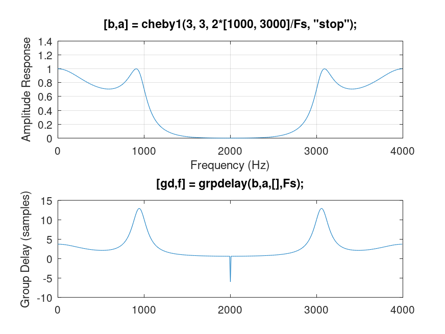
 % IIR bandstop filter has delays at [1000, 3000]
 %--------------------------------------------------------------
 Fs = 8000;
 [b, a] = cheby1(3, 3, 2*[1000, 3000]/Fs, 'stop');
 [H,f] = freqz(b,a,[],Fs);
 [gd,f] = grpdelay(b,a,[],Fs);
 subplot(211);
 plot(f,abs(H));
 title('[b,a] = cheby1(3, 3, 2*[1000, 3000]/Fs, "stop");');
 xlabel('Frequency (Hz)');
 ylabel('Amplitude Response');
 grid('on');
 subplot(212);
 plot(f,gd);
 title('[gd,f] = grpdelay(b,a,[],Fs);');
 ylabel('Group Delay (samples)');
Produces the following output
warning: grpdelay: setting group delay to 0 at singularity
warning: called from
    grpdelay at line 191 column 5
    get_output at line 50 column 5
    __html_help_text__ at line 67 column 28
    generate_package_html>wrote_html at line 869 column 5
    generate_package_html at line 211 column 13

warning: grpdelay: setting group delay to 0 at singularity
warning: called from
    grpdelay at line 191 column 5
    get_output at line 50 column 5
    __html_help_text__ at line 67 column 28
    generate_package_html>wrote_html at line 869 column 5
    generate_package_html at line 211 column 13
and the following figure
| Figure 1 |
|---|
 |
Package: signal