- Function File:
[B,A] =invfreqs(H,F,nB,nA) ¶ - :
[B,A] =invfreqs(H,F,nB,nA,W) ¶ - :
[B,A] =invfreqs(H,F,nB,nA,W,iter,tol,'trace') ¶ Fit filter B(s)/A(s)to the complex frequency response H at frequency points F.
A and B are real polynomial coefficients of order nA and nB.
Optionally, the fit-errors can be weighted vs frequency according to the weights W.
Note: all the guts are in invfreq.m
H: desired complex frequency response
F: frequency (must be same length as H)
nA: order of the denominator polynomial A
nB: order of the numerator polynomial B
W: vector of weights (must be same length as F)
Example:
      B = [1/2 1];
      A = [1 1];
      w = linspace(0,4,128);
      H = freqs(B,A,w);
      [Bh,Ah] = invfreqs(H,w,1,1);
      Hh = freqs(Bh,Ah,w);
      plot(w,[abs(H);abs(Hh)])
      legend('Original','Measured');
      err = norm(H-Hh);
      disp(sprintf('L2 norm of frequency response error = %f',err));
Demonstration 1
The following code
B = [1/2 1];
B = [1 0 0];
A = [1 1];
##A = [1 36 630 6930 51975 270270 945945 2027025 2027025]/2027025;
A = [1 21 210 1260 4725 10395 10395]/10395;
A = [1 6 15 15]/15;
w = linspace(0, 8, 128);
H0 = freqs(B, A, w);
Nn = (randn(size(w))+j*randn(size(w)))/sqrt(2);
order = length(A) - 1;
[Bh, Ah, Sig0] = invfreqs(H0, w, [length(B)-1 2], length(A)-1);
Hh = freqs(Bh,Ah,w);
[BLS, ALS, SigLS] = invfreqs(H0+1e-5*Nn, w, [2 2], order, [], [], [], [], "method", "LS");
HLS = freqs(BLS, ALS, w);
[BTLS, ATLS, SigTLS] = invfreqs(H0+1e-5*Nn, w, [2 2], order, [], [], [], [], "method", "TLS");
HTLS = freqs(BTLS, ATLS, w);
[BMLS, AMLS, SigMLS] = invfreqs(H0+1e-5*Nn, w, [2 2], order, [], [], [], [], "method", "QR");
HMLS = freqs(BMLS, AMLS, w);
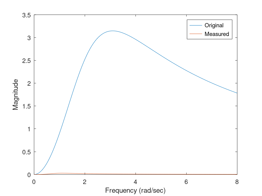
plot(w,[abs(H0); abs(Hh)])
xlabel("Frequency (rad/sec)");
ylabel("Magnitude");
legend('Original','Measured');
err = norm(H0-Hh);
disp(sprintf('L2 norm of frequency response error = %f',err));
Produces the following output
L2 norm of frequency response error = 26.323872
and the following figure
| Figure 1 |
|---|
 |
Package: signal