- Function File:
[B,A] =invfreqz(H,F,nB,nA) ¶ - :
[B,A] =invfreqz(H,F,nB,nA,W) ¶ - :
[B,A] =invfreqz(H,F,nB,nA,W,iter,tol,'trace') ¶ Fit filter B(z)/A(z)to the complex frequency response H at frequency points F.
A and B are real polynomial coefficients of order nA and nB. Optionally, the fit-errors can be weighted vs frequency according to the weights W.
Note: all the guts are in invfreq.m
H: desired complex frequency response
F: normalized frequency (0 to pi) (must be same length as H)
nA: order of the denominator polynomial A
nB: order of the numerator polynomial B
W: vector of weights (must be same length as F)
Example:
    [B,A] = butter(4,1/4);
    [H,F] = freqz(B,A);
    [Bh,Ah] = invfreq(H,F,4,4);
    Hh = freqz(Bh,Ah);
    disp(sprintf('||frequency response error||= %f',norm(H-Hh)));
Demonstration 1
The following code
order = 9; # order of test filter
# going to 10 or above leads to numerical instabilities and large errors
fc = 1/2; # sampling rate / 4
n = 128; # frequency grid size
[B0, A0] = butter(order, fc);
[H0, w] = freqz(B0, A0, n);
Nn = (randn(size(w))+j*randn(size(w)))/sqrt(2);
[Bh, Ah, Sig0] = invfreqz(H0, w, order, order);
[Hh, wh] = freqz(Bh, Ah, n);
[BLS, ALS, SigLS] = invfreqz(H0+1e-5*Nn, w, order, order, [], [], [], [], "method", "LS");
HLS = freqz(BLS, ALS, n);
[BTLS, ATLS, SigTLS] = invfreqz(H0+1e-5*Nn, w, order, order, [], [], [], [], "method", "TLS");
HTLS = freqz(BTLS, ATLS, n);
[BMLS, AMLS, SigMLS] = invfreqz(H0+1e-5*Nn, w, order, order, [], [], [], [], "method", "QR");
HMLS = freqz(BMLS, AMLS, n);
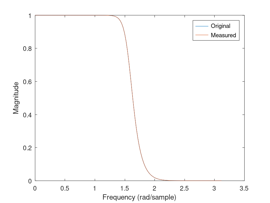
plot(w,[abs(H0) abs(Hh)])
xlabel("Frequency (rad/sample)");
ylabel("Magnitude");
legend('Original','Measured');
err = norm(H0-Hh);
disp(sprintf('L2 norm of frequency response error = %f',err));
Produces the following output
L2 norm of frequency response error = 0.000000
and the following figure
| Figure 1 |
|---|
 |
Package: signal