- Function File:
a =lpc(x)¶ - Function File:
a =lpc(x, p)¶ - Function File:
[a, g] =lpc(…)¶ - Function File:
[a, g] =lpc(x, p)¶ -
Determines the forward linear predictor by minimizing the prediction error in the least squares sense. Use the Durbin-Levinson algorithm to solve the Yule-Walker equations obtained by the autocorrelation of the input signal.
x is a data vector used to estimate the lpc model of p-th order, given by the prediction polynomial
a = [1 a(2) …
a(p+1)]
. If p is not provided,length(p) - 1is used as default.x might also be a matrix, in which case each column is regarded as a separate signal.
lpcwill return a model estimate for each column of x.g is the variance (power) of the prediction error for each signal in x.
See also: aryule,levinson.
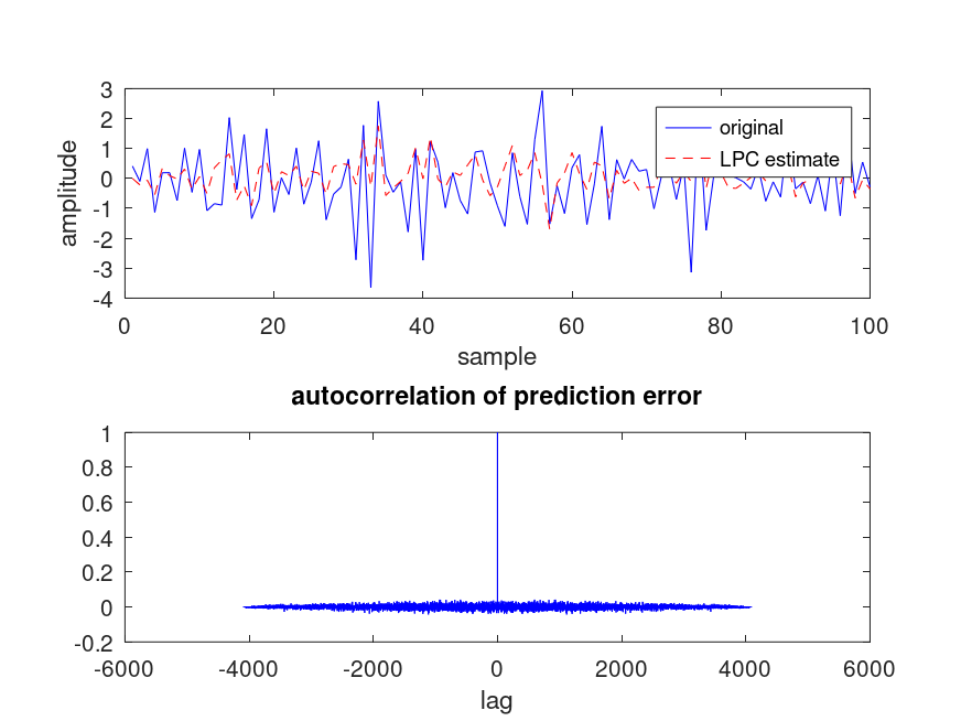
Demonstration 1
The following code
 noise = randn (10000, 1);
 x = filter (1, [1 1/2 1/4 1/8], noise);
 x = x(end-4096:end);
 [a, g] = lpc (x, 3);
 xe = filter ([0 -a(2:end)], 1, x);
 e = x - xe;
 [ac, k] = xcorr (e, "coeff");
 subplot (2,1,1); plot (x(1:100), "b-", xe(1:100), "r--");
 xlabel ("sample"); ylabel ("amplitude"); legend ("original","LPC estimate");
 subplot (2,1,2); plot (k,ac,"b-"); xlabel ("lag");
 title ("autocorrelation of prediction error");
Produces the following figure
| Figure 1 |
|---|
 |
Demonstration 2
The following code
 if !isempty ( pkg ("list", "ltfat") )
   pkg load ltfat
   [sig, fs] = linus;
   x = sig(13628:14428);
   [a, g] = lpc (x, 8);
   F = round (sort (unique (abs (angle (roots (a))))) * fs / (2 * pi) );
   [h, w] = freqz (1, a, 512, "whole");
   subplot (2, 1, 1);
   plot ( 1E3 * [0:1/fs:(length (x)-1)*1/fs], x);
   xlabel ("time (ms)"); ylabel ("Amplitude");
   title ( "'linus' test signal" );
   subplot (2, 1, 2);
   plot (w(1:256)/pi, 20*log10 (abs (h(1:256))));
   xlabel ("Normalized Frequency ({\\times \\pi} rad/sample)")
   ylabel ("Magnitude (dB)")
   txt = sprintf (['Signal sampling rate = %d kHz\nFormant frequencies: ' ...
      '\nF1 = %d Hz\nF2 = %d Hz\nF3 = %d Hz\nF4 = %d Hz'], fs/1E3, ...
      F(1), F(2), F(3), F(4));
   text (0.6, 20, txt);
 endif
 ## test input validation
gives an example of how 'lpc' is used.
Package: signal