- Function File:
[rmsx,w] =movingrms(x,w,rc,Fs=1)¶ Calculate moving RMS value of the signal in x.
The signal is convoluted against a sigmoid window of width w and risetime rc. The units of these parameters are relative to the value of the sampling frequency given in Fs (Default value = 1).
Run
demo movingrmsto see an example.See also: sigmoid_train.
Demonstration 1
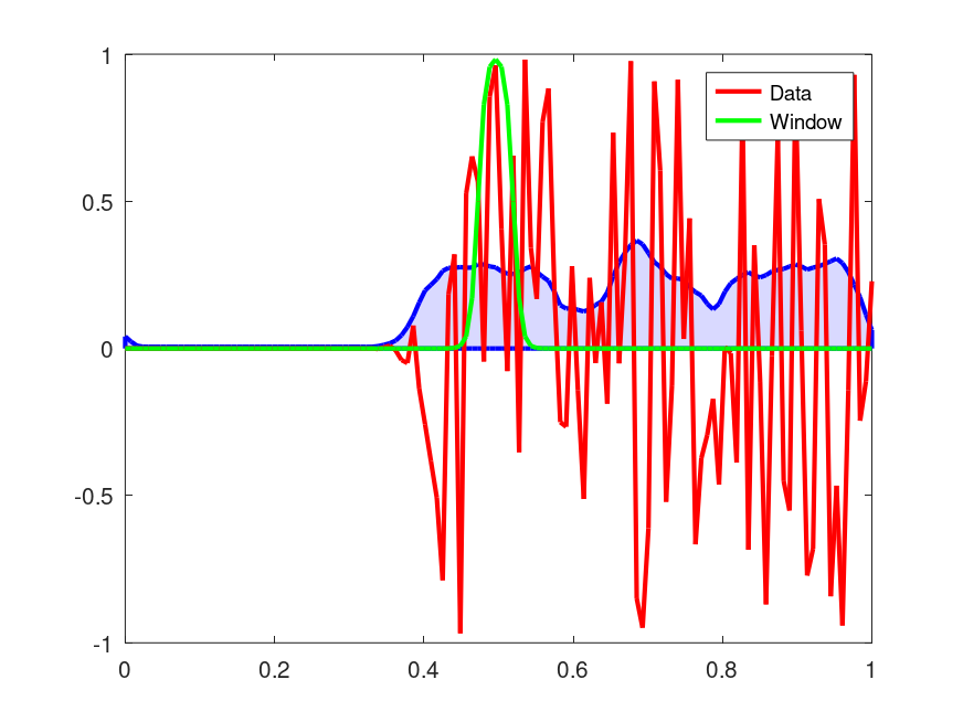
The following code
 N = 128;
 t = linspace(0,1,N)';
 x = sigmoid_train (t,[0.4 inf],1e-2).*(2*rand(size(t))-1);
 Fs    = 1/diff(t(1:2));
 width = 0.05;
 rc = 5e-3;
 [wx w] = movingrms (zscore (x),width,rc,Fs);
 area (t,wx,'facecolor',[0.85 0.85 1],'edgecolor','b','linewidth',2);
 hold on;
 h = plot (t,x,'r-;Data;',t,w,'g-;Window;');
 set (h, 'linewidth', 2);
 hold off;
 # ---------------------------------------------------------------------------
 # The shaded plot shows the local RMS of the Data: white noise with onset at
 # aprox. t== 0.4.
 # The observation window is also shown.
Produces the following figure
| Figure 1 |
|---|
 |
Demonstration 2
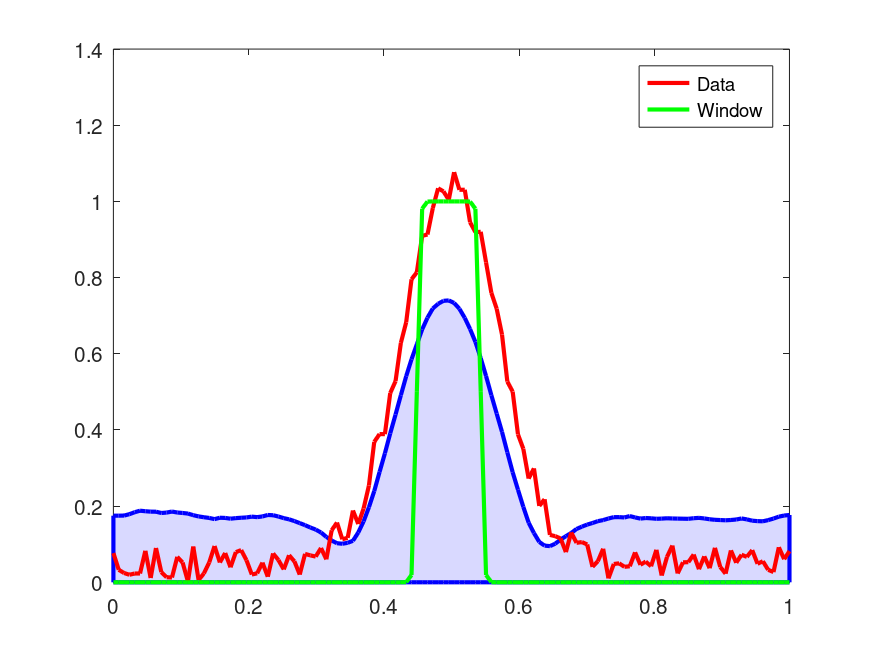
The following code
 N = 128;
 t = linspace(0,1,N)';
 x = exp(-((t-0.5)/0.1).^2) + 0.1*rand(N,1);
 Fs    = 1/diff(t(1:2));
 width = 0.1;
 rc = 2e-3;
 [wx w] = movingrms (zscore (x),width,rc,Fs);
 area (t,wx,'facecolor',[0.85 0.85 1],'edgecolor','b','linewidth',2);
 hold on;
 h = plot (t,x,'r-;Data;',t,w,'g-;Window;');
 set (h, 'linewidth', 2);
 hold off;
 # ---------------------------------------------------------------------------
 # The shaded plot shows the local RMS of the Data: Gausian with centered at
 # aprox. t== 0.5.
 # The observation window is also shown.
Produces the following figure
| Figure 1 |
|---|
 |
Package: signal