Function File: [psd,f_out] = pburg(x, poles, freq, Fs, range, method, plot_type, criterion) ¶

Calculate Burg maximum-entropy power spectral density.

The functions "arburg" and "ar_psd" do all the work. See "help arburg" and "help ar_psd" for further details.

ARGUMENTS:

All but the first two arguments are optional and may be empty.

x

[vector] sampled data

poles

[integer scalar] required number of poles of the AR model

freq

[real vector] frequencies at which power spectral density is calculated.

[integer scalar] number of uniformly distributed frequency values at which spectral density is calculated. [default=256]

Fs

[real scalar] sampling frequency (Hertz) [default=1]

CONTROL-STRING ARGUMENTS – each of these arguments is a character string.

Control-string arguments can be in any order after the other arguments.

range

’half’, ’onesided’ : frequency range of the spectrum is from zero up to but not including sample_f/2. Power from negative frequencies is added to the positive side of the spectrum.

’whole’, ’twosided’ : frequency range of the spectrum is -sample_f/2 to sample_f/2, with negative frequencies stored in "wrap around" order after the positive frequencies; e.g. frequencies for a 10-point ’twosided’ spectrum are 0 0.1 0.2 0.3 0.4 0.5 -0.4 -0.3 -0.2 -0.1

’shift’, ’centerdc’ : same as ’whole’ but with the first half of the spectrum swapped with second half to put the zero-frequency value in the middle. (See "help fftshift". If "freq" is vector, ’shift’ is ignored. If model coefficients "ar_coeffs" are real, the default range is ’half’, otherwise default range is ’whole’.

method

’fft’: use FFT to calculate power spectral density.

’poly’: calculate spectral density as a polynomial of 1/z N.B. this argument is ignored if the "freq" argument is a vector. The default is ’poly’ unless the "freq" argument is an integer power of 2.

plot_type

’plot’, ’semilogx’, ’semilogy’, ’loglog’, ’squared’ or ’db’: specifies the type of plot. The default is ’plot’, which means linear-linear axes. ’squared’ is the same as ’plot’. ’dB’ plots "10*log10(psd)". This argument is ignored and a spectrum is not plotted if the caller requires a returned value.

criterion

[optional string arg] model-selection criterion. Limits the number of poles so that spurious poles are not added when the whitened data has no more information in it (see Kay & Marple, 1981). Recognized values are

’AKICc’ – approximate corrected Kullback information criterion (recommended),

’KIC’ – Kullback information criterion

’AICc’ – corrected Akaike information criterion

’AIC’ – Akaike information criterion

’FPE’ – final prediction error" criterion

The default is to NOT use a model-selection criterion

RETURNED VALUES:

If return values are not required by the caller, the spectrum is plotted and nothing is returned.

psd

[real vector] power-spectral density estimate

f_out

[real vector] frequency values

HINTS

This function is a wrapper for arburg and ar_psd.

See "help arburg", "help ar_psd".

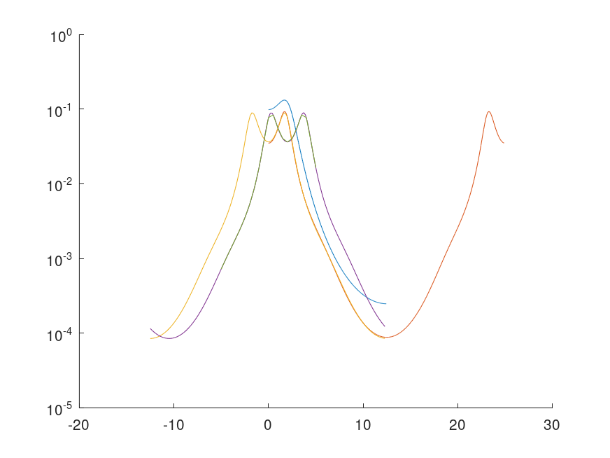
Demonstration 1

Package: signal