Function Reference: pulstran

Function File: y = pulstran (t, d, func, …) ¶

Function File: y = pulstran (t, d, p) ¶

Function File: y = pulstran (t, d, p, Fs) ¶

Function File: y = pulstran (t, d, p, Fs, method) ¶

Generate the signal y=sum(func(t+d,...)) for each d. If d is a matrix of two columns, the first column is the delay d and the second column is the amplitude a, and y=sum(a*func(t+d)) for each d,a. Clearly, func must be a function which accepts a vector of times. Any extra arguments needed for the function must be tagged on the end.

Example:

fs = 11025;  # arbitrary sample rate
f0 = 100;    # pulse train sample rate
w = 0.001;   # pulse width of 1 millisecond
auplot (pulstran (0:1/fs:0.1, 0:1/f0:0.1, "rectpuls", w), fs);

If instead of a function name you supply a pulse shape sampled at frequency Fs (default 1 Hz), an interpolated version of the pulse is added at each delay d. The interpolation stays within the the time range of the delayed pulse. The interpolation method defaults to linear, but it can be any interpolation method accepted by the function interp1.

Example:

fs = 11025;      # arbitrary sample rate
f0 = 100;        # pulse train sample rate
w = boxcar(10);  # pulse width of 1 millisecond at 10 kHz
auplot (pulstran (0:1/fs:0.1, 0:1/f0:0.1, w, 10000), fs);

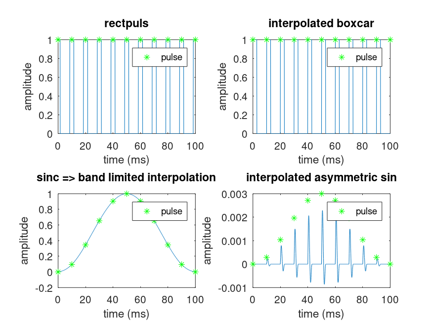
Demonstration 1

The following code

 fs = 11025;                   # arbitrary sample rate
 f0 = 100;                     # pulse train sample rate
 w = 0.003;                    # pulse width of 3 milliseconds
 t = 0:1/fs:0.1; d=0:1/f0:0.1; # define sample times and pulse times
 a = hanning(length(d));       # define pulse amplitudes

 subplot(221);
 x = pulstran(t', d', 'rectpuls', w);
 plot([0:length(x)-1]*1000/fs, x);
 hold on; plot(d*1000,ones(size(d)),'g*;pulse;'); hold off;
 ylabel("amplitude"); xlabel("time (ms)");
 title("rectpuls");

 subplot(223);
 x = pulstran(f0*t, [f0*d', a], 'sinc');
 plot([0:length(x)-1]*1000/fs, x);
 hold on; plot(d*1000,a,'g*;pulse;'); hold off;
 ylabel("amplitude"); xlabel("time (ms)");
 title("sinc => band limited interpolation");

 subplot(222);
 pulse = boxcar(30);  # pulse width of 3 ms at 10 kHz
 x = pulstran(t, d', pulse, 10000);
 plot([0:length(x)-1]*1000/fs, x);
 hold on; plot(d*1000,ones(size(d)),'g*;pulse;'); hold off;
 ylabel("amplitude"); xlabel("time (ms)");
 title("interpolated boxcar");

 subplot(224);
 pulse = sin(2*pi*[0:0.0001:w]/w).*[w:-0.0001:0];
 x = pulstran(t', [d', a], pulse', 10000);
 plot([0:length(x)-1]*1000/fs, x);
 hold on; plot(d*1000,a*w,'g*;pulse;'); hold off; title("");
 ylabel("amplitude"); xlabel("time (ms)");
 title("interpolated asymmetric sin");

 %----------------------------------------------------------
 % Should see (1) rectangular pulses centered on *,
 %            (2) rectangular pulses to the right of *,
 %            (3) smooth interpolation between the *'s, and
 %            (4) asymmetric sines to the right of *

Produces the following figure

Figure 1

Package: signal