- Function File:
[y s] =sigmoid_train(t, ranges, rc)¶ -
Evaluate a train of sigmoid functions at t.
The number and duration of each sigmoid is determined from ranges. Each row of ranges represents a real interval, e.g. if sigmoid
istarts att=0.1and ends att=0.5, thenranges(i,:) = [0.1 0.5]. The input rc is an array that defines the rising and falling time constants of each sigmoid. Its size must equal the size of ranges.The individual sigmoids are returned in s. The combined sigmoid train is returned in the vector y of length equal to t, and such that
Y = max (S).Run
demo sigmoid_trainto some examples of the use of this function.
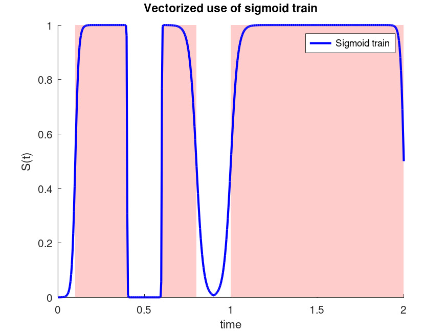
Demonstration 1
The following code
 # Vectorized
 t     = linspace (0, 2, 500);
 range = [0.1 0.4; 0.6 0.8; 1 2];
 rc    = [1e-2 1e-3; 1e-3 2e-2; 2e-2 1e-2];
 y     = sigmoid_train (t, range, rc);
 for i=1:3
     patch ([range(i,[2 2]) range(i,[1 1])], [0 1 1 0],...
               'facecolor', [1 0.8 0.8],'edgecolor','none');
 endfor
 hold on; plot (t, y, 'b;Sigmoid train;','linewidth',2); hold off
 xlabel('time'); ylabel('S(t)')
 title ('Vectorized use of sigmoid train')
 axis tight
 #-------------------------------------------------------------------------
 # The colored regions show the limits defined in range.
Produces the following figure
| Figure 1 |
|---|
 |
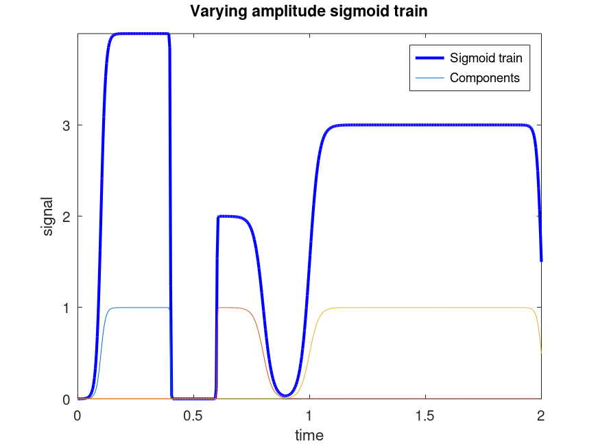
Demonstration 2
The following code
 # Varaible amplitude
 t     = linspace (0, 2, 500);
 range = [0.1 0.4; 0.6 0.8; 1 2];
 rc    = [1e-2 1e-3; 1e-3 2e-2; 2e-2 1e-2];
 amp   = [4 2 3];
 [~, S] = sigmoid_train (t, range, rc);
 y = amp * S;
 h = plot (t, y, '-b', t, S, '-');
 set (h(1), "linewidth", 2);
 legend (h(1:2), {"Sigmoid train", "Components"});
 xlabel('time'); ylabel('signal')
 title ('Varying amplitude sigmoid train')
 axis tight
Produces the following figure
| Figure 1 |
|---|
 |
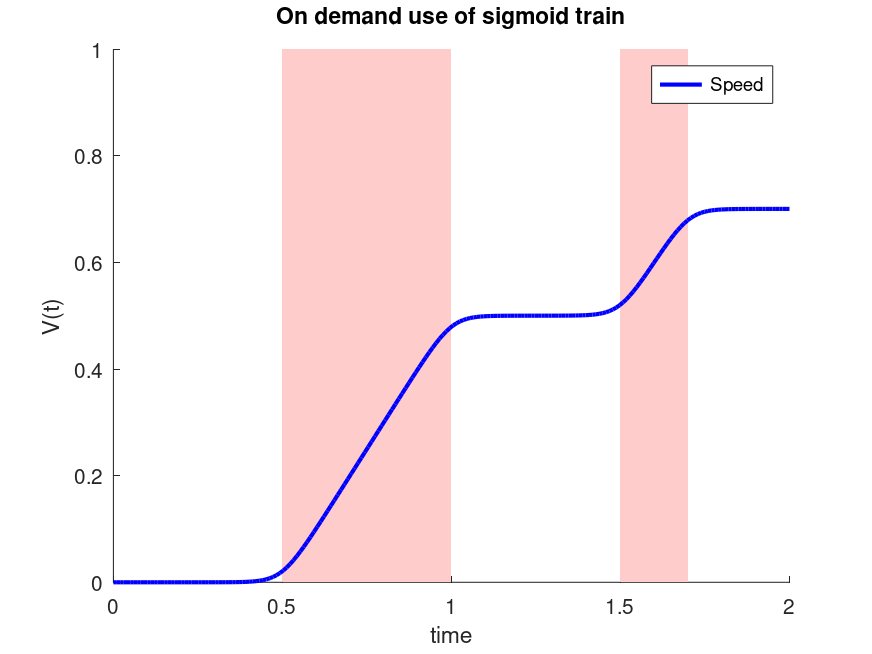
Demonstration 3
The following code
 # On demand
 t = linspace(0,2,200).';
 ran = [0.5 1; 1.5 1.7];
 rc = 3e-2;
 dxdt = @(x_,t_) [ x_(2); sigmoid_train(t_, ran, rc) ];
 y = lsode(dxdt,[0 0],t);
 for i=1:2
     patch ([ran(i,[2 2]) ran(i,[1 1])], [0 1 1 0],...
               'facecolor', [1 0.8 0.8],'edgecolor','none');
 endfor
 hold on; plot (t, y(:,2), 'b;Speed;','linewidth',2); hold off
 xlabel('time'); ylabel('V(t)')
 title ('On demand use of sigmoid train')
 axis tight
 #-------------------------------------------------------------------------
 # The colored regions show periods when the force is active.
Produces the following figure
| Figure 1 |
|---|
 |
Package: signal